Shack-Hartmann recipe
The following recipe is for carrying out and analysing Shack-Hartmann tests
at the WHT. The procedure should be similar for the INT (see Section 7).
Allow one hour to obtain Shack-Hartmann data at two elevations (e.g. 90
and 30 deg), and about 15 minutes to reduce the data from each test.
Occasional users of the Shack-Hartmann camera will probably find it
more helfpul to skip to the summary on the
Shack-Hartmann occasional-users page,
which also happens to be more up-to-date with
regard to the acquisition camera.
Contents:
- A few days before the camera is to be mounted
- Afternoon activities
- In twilight
- At night
- Data analysis
- Interpretation
- Shack-Hartmann tests at the INT
- Acknowledgments
- Check that all components have been located:
| A - | telescope interface + spacer ring
| | B - | acquisition / calibration section
| | C - | collimator-lens section
| | D - | mask, filter and shutter section
|
- Check that the
Fisher/Worswick technical manual is available
(used mainly for setup).
- Check that directory /data/qc/shack is visible.
- Check that an ubunto-unix computer is available,
for running the data-reduction software (prior to March 2018, the software
required a fedora-unix computer).
- Run through a test reduction of some old data,
e.g. runs teststar.fit and testlamp.fit
in /data/qc/shack/test. Data from previous Shack-Hartmann observations
can be found in the dated directories /data/qc/shack/yymmdd.
Most of steps 1 - 8 below are carried out by the OPS team, but don't
assume that all will be.
- Put the Shack-Hartmann camera somewhere accessible
on the observing floor
or in the control room
(not on the WHT ACAM port), with a monitor showing the output from
the TV camera.
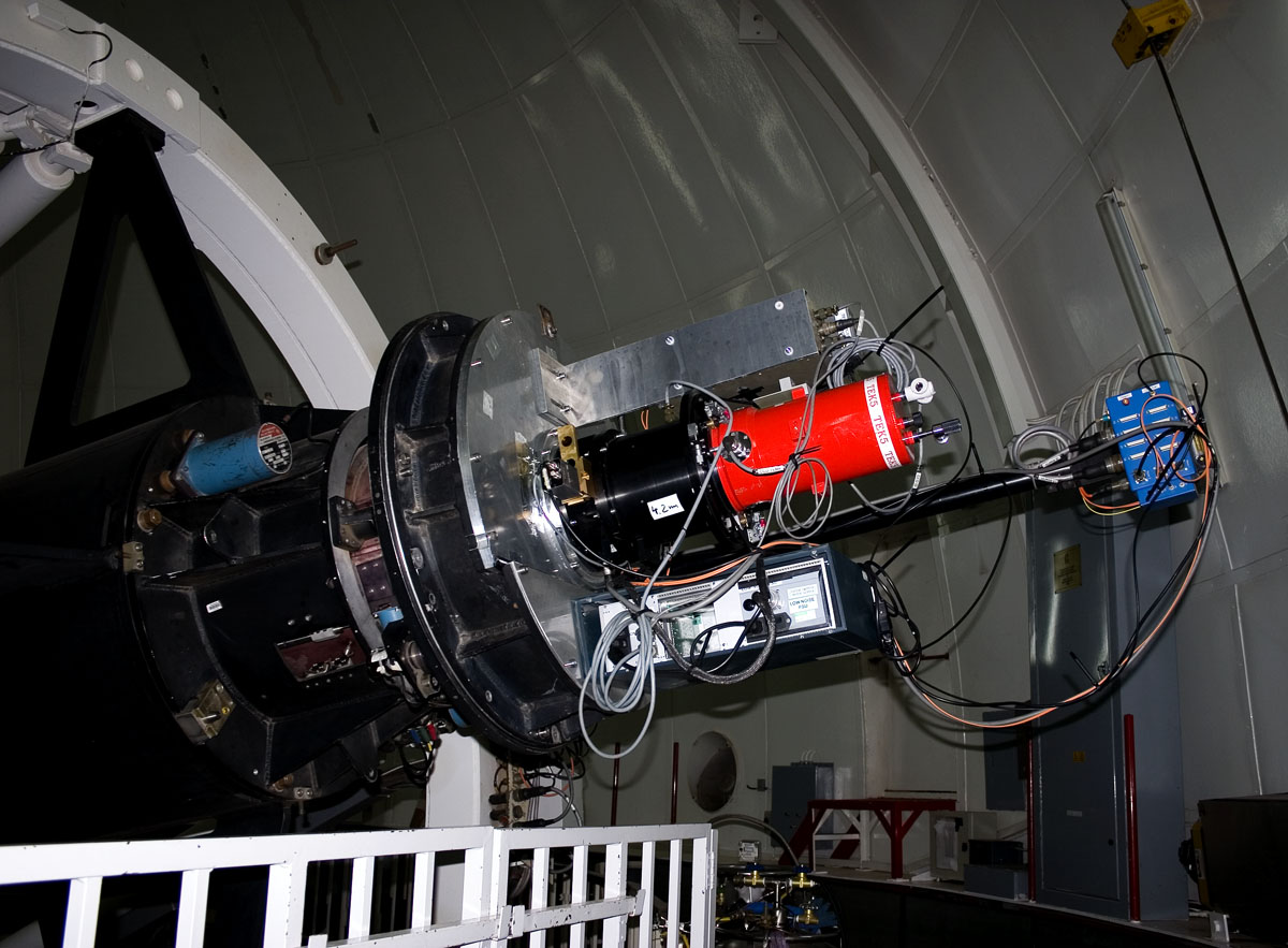
-
Move the blue filter into the TV path, i.e. move the
slide (which is quite stiff) to its lowest position as viewed
with the camera oriented in the position
in the photo
below. Don't use the central slide position - this is a green filter,
which has very different focus.
-
Note that the 3 25-mm filters in the slide in the light path to the TV have the same
central wavelengths as the 3 50-mm filters available for mounting in the
light path through the Shack-Hartmann camera:
433 (blue), 504 (blue-green) and 577 (yellow-green) nm.
Shack-Hartmann observations are usually made with blue filters in both
light paths (to maximise sensitivity to aberrations) and changing the
filter in the Shack-Hartmann light path requires partial dismantling of the camera (i.e. daytime only).
- Switch on the power supply for the lamp - usually two boxes left on
the desk in the control room.
Both boxes must be switched on (because the TV-control box runs the
fan for the lamp).
The boxes must be switched on (or off) in the order stated on the labels
on the front.
- Set the lamp current (top right knob) to about 2.8 Amps (voltage will
be ~ 5.7 V?).
- Release the two clamping
bolts on the TV slide (2.5-mm Allen key needed, NB the central locking screw
mentioned in the manual seems not to exist). Focus by moving the slide to
minimise the size of the image on the TV. Reclamp.
-
Mark the position of the lamp spot on the TV screen
(this where stars should be acquired). Beware parallax - stand in front
of the screen when making the mark.
- If the bulb fails, you'll need to remove 4 bolts holding the lamp housing
(spare bulbs in instrument-store cupboard).
- Mount the Shack-Hartmann unit (4 sections) on the required focal station
(section 3 of the manual), with a standard CCD as detector.
Hair and dust should be cleaned off the CCD window before the cryostat
is mounted.
Beware accidental 120-deg rotation of the CCD. TEK1 and TEK2 both
need the filler tube on the right, i.e. at 3 o'clock:
 Check that the lamp spot is still on the TV screen.
- Set CCD readout speed = 'Fast', no binning, no windowing.
- Make a trial exposure with e.g.:
run testinstrument 5
(The name was changed from aux2 to testinstrument in May 2016.)
-
Determine the exposure time needed to obtain a lamp frame with
maximum counts ~ 30000 (~ 6 sec in 2/2012, 20 sec in 5/2016 for
Cass; ~ 1 sec for WHT PF in 5/14).
-
Rotate the CCD so that the spots run along rows and columns,
with tilt < 4 pixels across the whole frame (NB the rows and columns
are not quite orthogonal, there's a rotation of ~ 0.2 dge between them,
i.e. ~ 3 in a 1000 pixels).
-
To rotate the CCD, you need to loosen the 4 bolts holding it to the
end plate of the Shack-Hartmann camera (Allen key and spanner needed).
These bolts are short, don't loosen them too much!
- Past settings in rotation (vernier D) at Cass ACAM/aux port were
3.1 for TEK1, and
5.5 for TEK2 5/2016.
At PF, D = 8.0 was OK for TEK1, but for TEK2 in 5/2014, it was not
possible to rotate the CCD enough for accurate alignment.
- When inspecting the lamp frame after adjusting the rotation of
the CCD, it's helpful to note that the small representation of the
image at the upper right of the ds9 display is sensitive to any
rotation of the spot pattern relative to the CCD rows and columns.
When there's significant rotation, this representation
shows a regular array
of circles. As the rotation is reduced, the circles expand and
decrease in number.
- When you're happy with the rotation, slacken off the
rotation vernier (D), tighten the bolts on the cryostat, measure the
position in rotation (D).
NB removal and replacement of the cryostat on the kinematic mount
(e.g. to clear condensation) can result
in a small relative rotation of the CCD, but probably by only a few tenths
of a pixel at the edges of the illuminated area.
- Check that the distance between spots is approx 1 mm on the CCD,
which on TEK2 is ~ 42 (24-micron) pixels.
- If light from the lamp is detected on the TV, but not on the CCD,
the CCD is probably not responding properly, even if the bias
image appears normal (this happened 2/07). If the CCD is responding OK,
it should detect dome light scattered into the camera.
If you suspect a problem with the optics, ask the operations-team staff
to remove the
CCD, then look into the camera with your eye on-axis, roughly where
the CCD would be. With the calibration lamp on (and the dome lights
off), you should see a faint blue spot, square in shape.
-
If some of the central spots are missing or attenuated,
and the background is brighter in that region (this happened 12/02),
there may be
condensation on some of the optical surfaces.
Example exposure of lamp:
- Check on the TCS info pages that the 3 transducers monitoring
the position of the
secondary mirror (M2) are within range, i.e. have values between
minus and plus 100 microns.
- Do a 7-star CALIBRATE (usually). Any recent changes in the derived
index errors can help distinguish between different possible
causes of imperfect PSF e.g. displacement vs tilt of M1.
- Point the telescope to a bright star (e.g. from the pointing grid),
mag <~ 4.5 for Shack-Hartmann observations at Cassegrain.
Advise the telescope operator to assume INSTRUMENT = OWN, at the
telescope control system.
- Acquire the star on the Shack-Hartmnann
TV, at the position where the lamp spot
was detected.
The field of view of the TV at Cass is square (edges parallel to
edges of screen) ~ 20 arcsec x 20 arcsec. At PF the field is probably
(estimated September 2020) ~ 100 arcsec x 80 arcsec.
The scale on the WHT control-room monitor
is ~ 0.2 arcsec/mm. Star images are degraded towards
the edge of the field of view.
- Focus the telescope. With the Shack-Hartmann camera mounted
on the Cassegrain A&G box, the focus should be ~ 97.85 (found 5/2016),
similar to that for
other Cass instruments. (At prime focus, it will be
~ 88.0 mm.)
Focus by minimising
the diameter of the star on the TV.
- Take a test exposure (~ 10 sec) of the star.
Two example exposures are shown below.
On the left image, the secondary-support vanes run along rows
and columns, and are not easy to see.
On the right image, the vanes are rotated ~ 45 deg, and are easier to see.
Below: enlarged view of spots
along the shadow of the vane in the lower left part of the image above right.
- Rotate the instrument platform so that the spider vanes run along the
rows and columns
of the chip (then these areas can easily be masked out).
The spider
vanes may be difficult to see when nearly aligned (tip: stand back from
display and defocus your eyes or, equivalently, look at the small copy
of the image in the top right corner of the ds9 image display).
Note that the spider vanes are not exactly in a cross shape, they are
arranged more like this:
           |
           |
           |
   -----
          +
             -----
        |
        |
        |
Usually ROT MOUNT 0 is OK (ROT MOUNT 10 was needed in 2/2012).
- Switch tracking of rotator off.
- Pick a reference spot which is easy to find, e.g. this one
near the centre of the array:
- Determine the coordinate system on the CCD by offsetting the
star 10 arcsec in
azimuth, then zero in azimuth, 10 in elevation (if you offset both
at once, star will be vignetted). The direction of any observed
aberrations
with respect to the mirror can then be determined by measuring the
position of the reference spot.
With the Shack-Hartmann camera mounted on the ACAM port, and
with the rotator at mount position = 0, azimuth increases to upper
right on the CCD as conventionally displayed, and elevation increases
to lower right (i.e. both at ~ 45 deg to the x,y columns).
The Shack-Hartmann observations require seeing less than 2 arcsec.
They can be carried out in moonlight (as long as the moon is not very close)
but not in bright twilight, because pisafind translates the gradient in
the background into changes in spot position.
Dust and poor transparency are not a problem, as long as sufficient
counts are obtained (criteria below).
Repeat the next five steps at each of the desired positions
of the telescope, e.g. elevation
~ 80 (for a quick test), or
~ 80, 20 (testing for possible changes with elevation),
or ~ 80, 50, 20, 50, 80 (testing for hysteresis with elevation).
- Acquire a bright star (mag ~< 4.5 for WHT, at the ACAM port)
at the position on
the TV where the lamp spot appeared.
The star should be single, i.e. no other star within a few arcmin.
- The telescope should be tracking.
The rotator should be set to a
fixed mount position as above (e.g. ROT MOUNT 0) and NOT tracking.
- Take an exposure.
Check that most of the spots are present. (During the Dec 2002 tests,
many of the spots near the centre of the array were weak, and
embedded in a diffuse glow, perhaps as a result of condensation.)
The FWHM of the spots will usually be <~ 10 pixels (the FWHM due to
diffraction at the lenslets has FWHM ~ 6 pixels, i.e. 1 arcsec).
- No autoguiding is possible because the mount PA is fixed.
Instead, the telescope must be hand guided, i.e. the telescope operator
should check every few minutes that the star is within 1 arcsec
of the acquisition position on the TV. But it's better that
guiding corrections are not made
*during* an individual exposure.
- Take 2 - 3 exposures of the star, aiming for ~ 20000 counts peak signal
(about 50 sec for star mag ~ 4, 100 sec for mag ~ 4.5).
The exposures should be long enough to average out seeing variations
(i.e. > 10 sec).
If the star has a close companion (< few 10s arcsec) the
Shack-Hartmann image will be double - switch
to another star.
- Offset the telescope ~ 5 arcmin, switch
on the lamp and take a lamp exposure (see previous section).
Star exposures are useless without lamp exposures at the same position
of the telescope.
If the telescope is offset only a few 10s of arcsec, the lamp
exposure will be contaminated by light from the star.
- If imaging is available at another focus, obtain hardcopies of images
of a bright star sufficiently out of focus that the spider vanes are
clearly visible. Obtain one image either side of focus (by the same
amount).
A recipe for this can be found here.
These out-of-focus images should reveal any gross aberrations and
serve to confirm the results of the Shack-Hartmann analyses, but they
are not essential.
The Cass TV is probably not useful for this, because of the
aberrations in the TV optics, although in principle these could be taken
into account by taking taking a second pair of intra/extra-focal images
with the mount PA changed by 180 deg.
The Shack-Hartmann TV has better optical quality, but suffers from
worse vignetting.
- Record the seeing e.g. as measured by the RoboDIMM.
The data-analysis procedure for a given pair of star + lamp images
identifies the locations of the (typically ~ 400)
spots in each image
and, for each spot identified in both images, measure the x,y offset
between star and lamp data. The optical aberrations are
calculated from the resulting set of ~ 400 x,y vectors.
The data analysis
involves running the scripts SH_findspots, SH_redhart
and SH_newhart. These were provided by Javier Mendez (in March 2018)
to supersede the long-winded
procedure
previously required (archived on that link in case some of the
troubleshooting information remains relevant).
The scripts should run from any astronomy account on any ING ubuntu-unix computer.
They can't be run from whtobs, which doesn't allow the appropriate calls (from SH_findspots)
to the Starlink packages
convert, figaro and pisa.
Proceed as follows:
-
Work in any directory. Copy in a pair of star and lamp
observations. The names are usually of the form
riiiinnn.fit, where iiiinnn is a 7-digit number.
Example star and lamp frames can be found
in /data/qc/shack/test/teststar.fit and testlamp.fit.
If any of the following files are
not present, copy them across from /data/qc/shack:
- defaults.dat
-
whtab_parms.dat
-
whtc_parms.dat
(there are 2 versions, one for Cass, one for prime focus
- copy across either whtc_parms.dat_cass or whtc_parms.dat_pf
and rename as whtc_parms.dat)
-
The 4 scripts SH, SH_findspots, SH_redhart and SH_newhart from
/data/qc/shack/code_linux/SH_pipeline_ubuntu.
The .dat files are a copy of those originally
~optics/oldsunos/hartmann (retrieved by Don, 2/07).
The parameters in the .dat files are defined in the comments section
of the newhart code as follows,
and are reproduced below with typical values for the WHT added:
Aberration configuration file whtab_parms.dat:

- x (focus) shift (mm) = 200
- radius of curvature = -19000
- eccentricity = 0.99
- tilt (arcsec) = 118.5
- scale change = 0.0000439
- spherical aberration factor =0.0254
- Y and Z coma factor = 0.0367
- 0-90 and 45-135 astigmatism factor = 0.0468

Optical_configuration_file whc_parms.dat:

- PRIME or CASSegrain focus = 1 for Prime, 2 for Cass
- Telescope aperture (mm) = 4180
- Primary radius of curvature (mm) = 23506 for Prime, 20879 for Cass
- Asphericity of primary = 1
- Separation between primary and secondary (mm) = 8.0350397e3
- Secondary radius of curvature (mm) = 6.2314e3
- Asphericity of secondary = 2.5329
- Telescope focus error - i.e. the amount to be added to the
  nominal primary-secondary spacing at a given focus position (mm) = 0.0
- Focal length of telescope (mm) = 11753 for Prime, 45738 for Cass
- Focal length of collimating lens in Hartmann system (mm)= 59 for Prime,
  260 for Cass
- Distance between Hartmann screen and detector (mm) = 170
- Detector pixel size (mm) = 0.024
Note that for the WHT, as indicated above, the following parameters in
whtc_parms.dat change betwen Prime and Cass: Prime or Cass flag;
Radius of curvature; Focal length of WHT; Focal length of Shack-Hartmann camera.
-
Check that the pixel size in mm (next to the last number in whtc_parms.dat)
is correct. If not, edit it.
-
Convert the raw observation of the star to the required format
and dynamic range, obtain the x,y positions of the spots
and (if an xterm is available) plot them:
- SH_findspots riiiinnn.fit
- SH_findspots asks 'Change displayed data range?'.
Reply 'y' if you want (unlikely) to change the x,y range of the data plotted
(usually ~ 1:1000, 1:1000) or the min, max (e.g. 0,3000).
- Use minpix typically 4 - 10 (usually 10),
method 0, background default, threshold
probably about 2000.
- SH_findpsots should find ~ 410 spots on the star image, ~ 540 on the lamp
image.
-
If the spot-finding fails with 'Internal storage space exhausted',
or, after a long pause, with a bus error,
it's probably finding too many objects, e.g. when the seeing is bad.
Try raising the threshold (e.g. doubling it).
- The x,y plot of the spot positions
shows whether the selection criteria for pisafind need changing.
On some computers (e.g. whtdrpc1) pisaplot works OK. On some,
it plots double size, so the overlay marks don't match up
with the light spots. Anyway, this step isn't critical
- it's just a sanity check.
- The spot positions are recorded in text file rnnn.dat
- Repeat the above steps for the lamp observation,
yielding spot-positions file rlll.dat (from raw data
riiiilll.fit).
- Match the positions listed in the two files rnnn.dat
(star frame) and rlll.dat (lamp frame), and measure the x,y differences:
- SH_redhart rnnn.dat rlll.dat
- Reply to the prompt for the focal station at which the data
were obtained (C = Cassegrain, P = prime).
- Reply to the prompt for the input data file names
(which default to the names given on the command line)
and the output file names (by default rednnn and hartnnn).
- SH_redhart will display the positions of the star spots
(circles) and lamp spots (dots) found by SH_findspots.
A visible offset dx, dy indicates that the star has not been
acquired at the
position of the lamp spot on the TV. The spots are 40 pixels apart,
scale ~ 0.16 arcsec/pixel, so if dx,dy (star position munus lamp position)
is >~ 3 arcsec, there may be problems
matching the correctly the star and lamp spots.
- Usually, you can accept the default scaling factor (1.0),
trial x and y shifts (0.0)
and search-box size (15), but if dx,dy (above) >~ 10 pixels, it will probably
help to use these as the trial x and y shifts (sign convention as
indicated above).
- Usually, SH_redhart matches every star spot to a lamp spot (i.e.
generates >~ 400 matches). If there are many missing, this could be
a sign of strong aberrations e.g. coma.
- To the question 'Plot or exit...', answer 'P',
otherwise it will not generate the
text file of vectors either.
- Give /vps as plot device.
- Select vector plot ('V') and accept the defaults for vector scaling (10),
and minimum and maximum x and y.
- There is an option 'Clean the image?' to
mask out spots whose centroids are affected by vignetting
near the inner or outer edge of the pupil (best to mask these)
or within four user-defined rectangles affected by the M2
support vanes (usually it's not necessary to mask these).
If you make a mistake during masking, there's an option at the end
to re-do them.
- The output files are rednnn, hartnnn and rednnn.ps.
Print rednnn and rednnn.ps.
Example vector plot, illustrating the need to mask out vectors near
the inner or outer circumference of the pupil:
- To derive the aberrations from the measured
shifts in file hartnnn:
- SH_newhart
- Accept the default names for the two telescope parameter files.
- Specify the spots and output filenames as hartnnn and newnnn.
- Give /vps as plot device.
- Print newnnn.ps and newnnn.
- If you prefer to run steps 3 - 5 above in one go, type:
SH riiiinnn.fit riiiilll.fit
where iiiinnn and iiiilll are the run numbers of the star and lamp images.
Then respond to the prompts as indicated above.
The vector plot (above)
shows the spot shifts remaining after the mean x,y shift
(movement of star) and mean radial expansion (focus shift) have been
removed. What is left is a superposition of the effects of spherical
aberration, astigmatism and coma, higher-order aberrations and random
terms.
Spherical aberration vectors point inwards or outwards, size increasing
(non-linearly) with radius from centre.
Astigmatism yields vectors pointing outwards at two opposite position
angles, and pointing inwards at the two position angles at 90 deg to
these. The vectors are larger at the edge than at the centre.
Coma yields vectors which point in the SAME direction at two opposite
position angles, and are zero at the two position angles at 90 deg to
these. Vector size goes as radius^2.
Bear in mind that even if one of these simple aberrations dominates,
the vectors will have had a mean radial-expansion term subtracted by
redhart.
Newhart interprets the vector pattern for you,
in terms of a superposition of the three simple low-order
aberrations. Newhart generates an output text file newnnn and
a plot file.
The text file reports the amplitude of the aberrations as
80% diameters and as rms (in mm and in arcsec).
Note that the FWHM of a cut through a 2-D Gaussian (i.e. a radially symmetric peak I(x,y) on the x,y plane) is
approximately 1.67 * rms. For the same shape, ee80 = 2.54 rms
or 1.52 FWHM.
The total rms is given about half way down the first page in x and y
directions. Even in the absence of higher-order aberrations, this is not
a simple quadratic sum of the individual rms given lower down the page
for spherical aberration, astigmatism and coma.
Coma is given as an extent as well as rms - the images look like an
axial slice through a cone. Coma is a signature of misalaignment between
primary and secondary mirrors, which can arise from relative tilt
or translation of either mirror. The aberration most often seen is
coma due to tilt of the primary mirror from its reference position.
The graphical output from newhart shows 8 plots. Plot 1 (upper left)
shows the sampling of the pupil.
Plots 2 - 4 show the raw spot pattern after subtracting focus,
after subtacting the 3 main aberrations,
and after subtracting coma only.
Plots 5-7 show the deduced contributions from spherical aberration,
coma and astigmatism. Plot 8 can be ignored.
Example plot from newhart:
The results from each Shack-Hartmann test are recorded in the
WHT optics log. Information about the
relationship between the newhart-quoted PA and azimuth/elevation,
can be found on the same page.

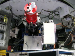
The Shack-Hartmann camera at INT prime focus in 2005 (photo by Javier Mendez,
click for full size)
When carrying out a Shack-Hartmann test at the Isaac Newton Telescope,
the procedure followed is similar to that at the WHT, but note, in particular,
the following differences:
- The interface flange and collimator section used depend on the
telescope and focal station (Section 1).
- The required telescope focus will for the INT be roughly ?? mm
(Section 3, item 5).
- The numerical parameters provided in the files intab_parms.dat
and intc_parms.dat (Section 5) are different [to be added].
The above notes are
based on: the Fisher/Worswick Shack-Hartmann manual; pre-1995 notes by
Vik Dhillon (setup) and Dave King (reduction);
experience since 1995
at the WHT; and comments from Marie Hrudkova in 2012.
Chris Benn
30 April 2002, last revised 13 June 2024
|