Back to the top

1. Mount the calcite analyser

   The calcite analyser (Fig. 1) should be mounted in the multi-slit position of the ISIS slit carriage. You may have to remove the image slicer first, which is present by default (ask for assistance from an optical engineer if you're not confident of doing this unaided). Note that the below-slit calcite slab (Savart plate) isn't used for imaging-polarimetry, but is only used for spectropolarimetry observations.
   
   First move the dichroic out of the beam for easy access:
   
   SYS@taurus> bfold 0
   
   Then, protect the slit unit with the dekker slide (note that it is necessary to have the dekker out, that is in position 1, in order to be able to open the slit door):
   
   SYS@taurus> dekker 1
   
   Now move the multi-slit unit into the light path. In order to have the correct information displayed in the ISIS Mimic, Instrument Control Console and image headers, select the ISIS Observer tab of the Instrument Control Console, and in the Slit Unit section choose the "Imaging polarimetry" option. This will move the multi-slit unit into the light path, and the image-header keyword ISISLITU will show IMAGE_POL.
   
   Next, unlock the slit door:
   
   SYS@taurus> slit_door open
   
   You can now physically open the slit door, located above the red cryostat. Inside you will have access to the slit unit, dichroic, filters and dekker. Carefully slide out the image slicer (if it was deployed in the multi-slit unit), put it in its box and store it in the WHT observing-floor cabinet. Take the analyser unit, also stored in the WHT observing-floor cabinet, out of its box, carefully slide it into position and tighten the bolt (see Fig. 2).
   
   If you want to change filters (see next section) proceed in a similar way with the filter units: just slide them out, put them back in their boxes and introduce the new ones in the unit. Be careful to slide them fully in, making sure they are properly seated.
   
   Physically close the slit door and then lock it:
   
   SYS@taurus> slit_door close
   
   You can leave the dekker in position 1 because in imaging polarimetry mode the dekker position does not matter - the dekker is always above the long slit, which is out of the light path.
   
   For observations with the blue arm the dichroic deployed should preferably be the D5300, with the bfold in the mirror position:
   
   SYS@taurus> bfold 1
   
   For observations with the red arm the dichroic should be out of the beam:
   
   SYS@taurus> bfold 0
   
   
   

   
   
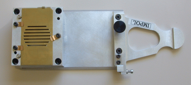
   Fig. 1 -  The analyser unit for imaging polarimetry. The unit should be mounted in the ISIS multi-slit position. The calcite is below the dekker field mask (shown in yellow).
   
   

   
   
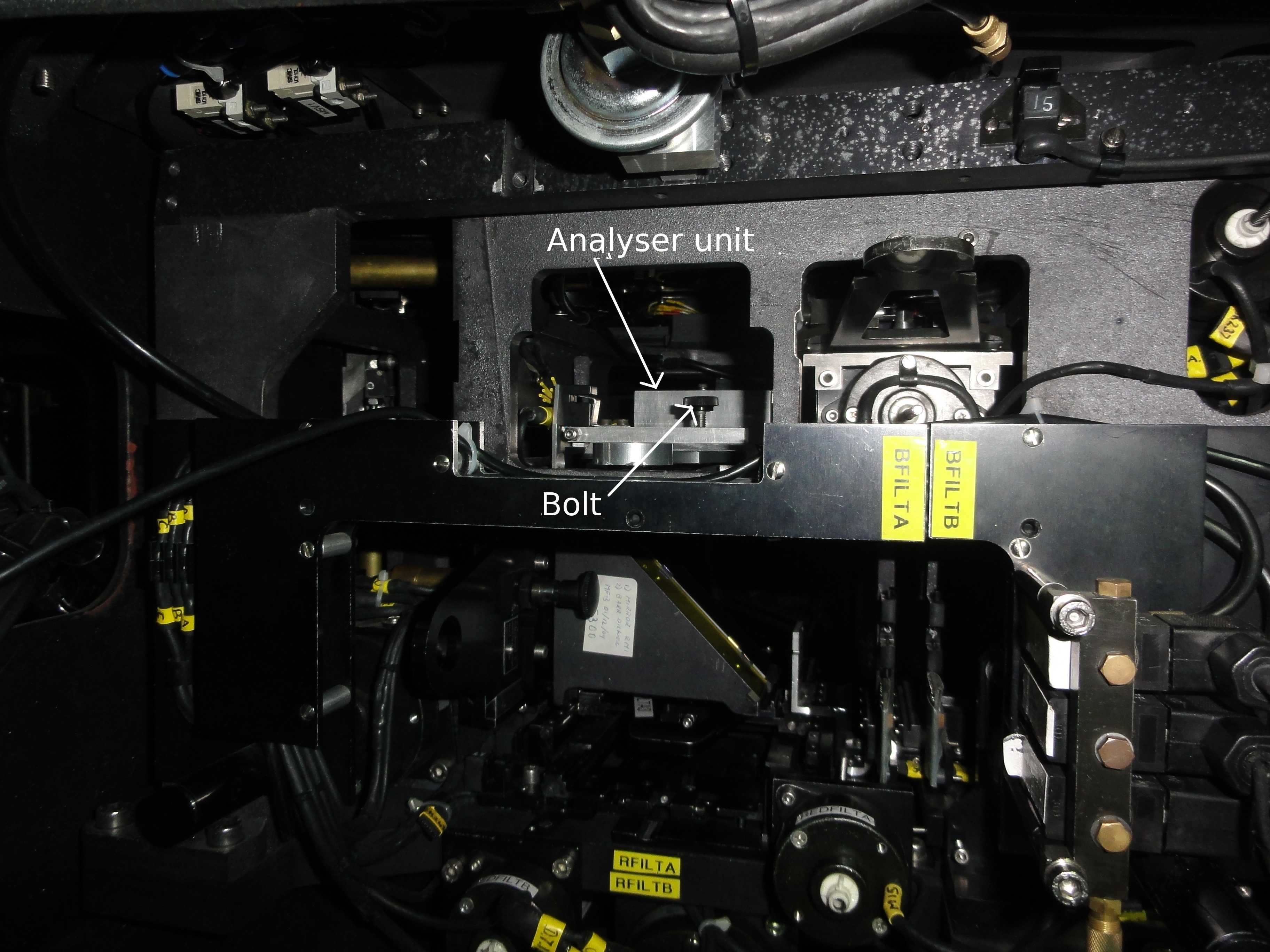
   Fig. 2 -  The position of the analyser unit inside the ISIS slit area. The analyser unit should be fixed in position by tightening the locking bolt.
   
   
2. Mount the filters
   

   Colour and/or neutral density filters have to be mounted in filter holders that were specially adapted for imaging-polarimetry observations (Fig. 3). These filter holders are designed to deploy 50x50-mm square filters, and can cater for some 50-mm circular filters too. Check in advance which filters are requested by the observer and thart they will fit in the available filter holders, or whether some modification has to be done (the filter thickness has to be taken into account too).

   The filter slides are then mounted in their position below the ISIS slit unit following the same procedure used to mount the analyser unit (it is a good idea to change the analyser and filters at the same time). Two filters can be mounted in each arm. Remember that it is recommended to use only one arm at a time for the imaging polarimetry observations.
   
   
   
   
   
   
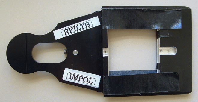
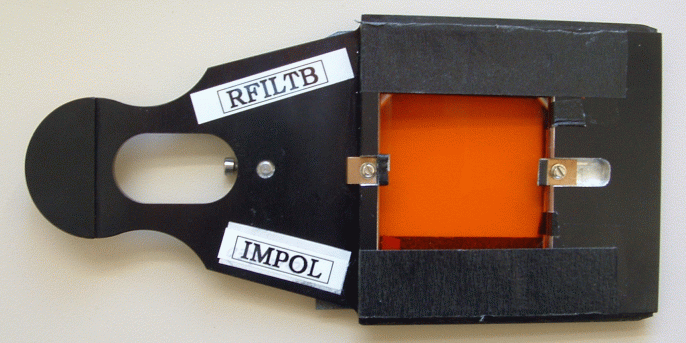
   Fig. 3 - Top: one of the two filter holders used for the red arm. Similar filter holders can be mounted in the blue arm. Bottom: R filter mounted in the filter holder. Notice that black masking tape at the sides of the 50x50-mm square filters is needed to avoid light leaks around their edges.
   
   Normal filter slides hold two filters, but the slides modified for imaging polarimetry can hold only one filter. For imaging polarimetry observations, filter position 4 should be used. Therefore, to use a filter mounted in the BFILTA (or BFILTB) slide type:
   
   SYS@taurus> bfilta 4 (or bfiltb 4)
   
   Similarly, to use a filter mounted in the RFILTA (or RFILTB) slide type:
   
   SYS@taurus> rfilta 4 (or rfiltb 4)
   
   Note that the slots for the RFILTA and RFILTB filter slides are located below the dichroic, while those for the BFILTA and BFILTB filter slides are located to the right side of the dichroic (see Fig. 2).
   
   When you've completed the filter changes, remember to update the filter database, indicating position number 4 for all filter slides deployed.
   

3. Mount the mirror

   The mirror should be mounted in the grating cell of the arm which is to be used for observations. Just replace the grating with the flat mirror unit in the same way as changing a grating. Any valid name of a grating works fine with the mirror as it will be used in order 0. So, for example, to change the red grating to the mirror you can type:
   
   SYS@taurus> setgrating red R1200R
   
   Then answer "yes" to access the grating-area door, and in the dome, open it manually. Release the grating as usual with the "open" button, deploy the mirror, use the "close" button and manually lock the grating-area door.
   
   Then set the central wavelength to 0:
   
   SYS@taurus> cenwave red  0
   
   Follow the same procedure if you need to put the mirror in the blue arm.
   
   If both arms of ISIS are going to be used, it is recommended to use the old mirror in the blue arm and the new mirror in the red arm (see here).



4. Put the retarder plate in the beam
   
   Deploy the halfwave plate (for linear polarimetry) or the quarterwave plate (for circular polarimetry) in the light path:
   
   SYS@taurus> hwin (for linear) or qwin (for circular)
   
   To take halfwave or quaterwave plate out of the beam, type:
   
   SYS@taurus> hwout or qwout
   


5. Setup the detector

   Setup ISIS to take a flat-field exposure:
   
   SYS@taurus> agcomp
   
   SYS@taurus> complamps w
   
   SYS@taurus> compnd 4
   
   In the red arm, a 1 sec exposure with this ND filter produced a flat-field like the one presented in Fig. 4, with enough counts to check the focus in a next step. In the blue arm, a 1 sec exposure with compnd 3 will produce similar flat field.
   
   Set the appropriate window and readout speed of the detector as usual.
   
   The windows below can be used as a reference. They cover the whole field of view and include an overscan region on the right side (see Fig. 4)
   
   For a linear polarimetry:
   
   SYS@taurus> window red 1 "[680:2148,1700:2470]"
   
   SYS@taurus> window blue 1 "[695:2148,1580:2440]"
   
   For a circular polarimetry:
   
   SYS@taurus> window red 1 "[770:2148,1820:2300]"
   
   SYS@taurus> window blue 1 "[800:2148,1750:2280]"
   
   
   
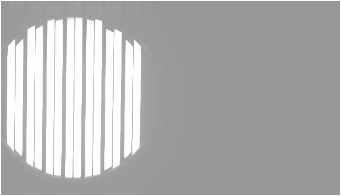
   Fig. 4 - This window includes the field and overscan columns of the CCD (right end of the image). The double pattern of slits corresponds to the ordinary and extra-ordinary image of the comb mask as produced by the calcite analyser.
   
   

6. Focus the spectrograph
   
   Set the collimator to a rough "nominal" focus using the commands:
   
   SYS@taurus> rcoll 9300 (for the red arm)
   
   SYS@taurus> bcoll 5100 (for the blue arm)

   Then make steps of r/bcoll values of 500 microns (the collimator units) around the nominal focus and take a flat-field exposure at each collimator value until the edges of the dekker are at their sharpest (as determined e.g. with IRAF-imexamine task), which will be the final collimator value. Use the same exposure time and ND filter as in the previous step. An example of flat fields taken at different spectrograph focuses (collimator values) is shown in Fig. 5.
   





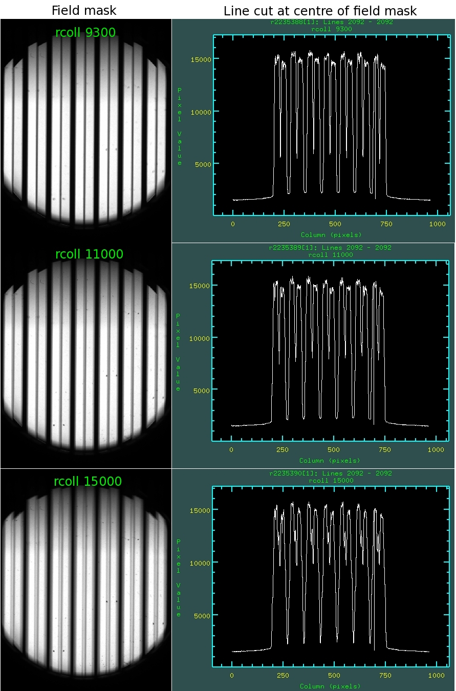
Fig. 5 -  Flat-field exposures at different collimator positions where spectrograph defocus can be seen. Top panels show images with a spectrograph in focus (rcoll 9300), middle panels show out-of-focus image (rcoll 11000) and bottom panels show even more out-of-focus image (rcoll 15000).


Find the instrumental zero angles

Zero angles are the angles of the retarder plate for which the contrast between the ordinary (o-) and extraordinary (e-) beams is maximized. The theoretical zero angles should be around 0 deg for a linear polarimetry and 90 deg for a circular polarimetry. However, zero angles in ISIS are known to have an offset. The table below summarizes the expected ISIS wave plate angles when doing linear and circular imaging-polarimetry observations.


ISIS arm	Polarimetry mode	Retarder	Angles (deg)
Red	Linear	Halfwave plate	8, 53, 30.5, 75.5
Red	Circular	Quarterwave plate	97, 187
Blue	Linear	Halfwave plate	11, 56, 33.5, 78.5
Blue	Circular	Quarterwave plate	97, 187

To find the instrumental zero angles insert the MF-POL-PAR filter in the beam:

SYS@taurus> mainfiltnd MF-POL-PAR

Now you should take flat-field images around the expected zero angle:

SYS@taurus> complamps w

SYS@taurus> hwp <angle> or qwp <angle>, to move the required plate to a requested angle between 0-360 deg

SYS@taurus> flat red 2 "angle"

To measure the average brightness use the central o- and e- rays. You can use the iraf imstat command on two rectangular regions, which must have the same size. For example:

cl> imstat r123456.fit[1][326:340,130:630]. For the o- ray.

cl> imstat r123456.fit[1][359:373,130:630]. For the e- ray.

Always use a fairly long region for good statistics on both rays. Take a note of the average count values and compute the difference. Do the same at remaining angles and record the angle of the maximum difference between both rays which will be the zero angle.

Linear polarisation (using the hwp plate)
Theoretically, for linear-polarisation observations, the target should be observed at the halfwave-plate angles 0, 45, 22.5, and 67.5 degrees. Hence, you should add +0, +45, +22.5, and +67.5 degrees to the zero angle you have found and use these angles for science observations by introducing them in the linear-polarimetry script at /home/whtobs/linimpolscript [1].

It is a good practice to check that other plate angles (+22.5, +45, and +67.5) make sense. With the half-wave plate at 22.5 and 67.5 deg away from the zero angle the difference in the intensity between the ordinary and extraordinary beams should be minimal, at 45 deg maximal.

Circular polarisation (using the qwp plate)
We were feeding the spectrograph with linearly polarised light when we measured a zero angle (we used the MF-POL-PAR), and therefore a final zero angle is obtained by adding 45 degrees to the measured angle. That is, if 52 degrees was the zero angle with the MF-POL-PAR, then the angle in the script for circular polarimetry should be 52+45=97 degrees. We will use this angle and +90 degrees in the circular-polarimetry script at /home/whtobs/cirimpolscript [1].

When you are finished, remember to remove the MF-POL-PAR filter out of the beam:

SYS@taurus> mainfiltnd out

Back to the top

Back to the top

Useful information

---

[1] These scripts are the same as for ISIS spectropolarimetry observations, except that for imaging polarimetry a waveplate does not move out of a beam during an acquisition.