 | |||
|

| Home > Astronomy > ACAM > The ACAM Acquisition Tool User's Guide |
The ACAM Acquisition Tool User's Guide
1. Introduction
This document is intended to provide a detailed guide for TOs and SAs
in the usage and calibration of the ACAM
Acquisition Tool. For a quick overview of the acquisition procedure, please refer to the section 'Example Acquisition Scenarios'. It currently outlines the strategy for performing spectroscopic target acquisition of a single object. (Advice for alternative observing scenarios will be added in the future.) 2. Overview of the ACAM Acquisition Procedure
| |||||||||||||||||||||||||||||||||||||||||
| Instrument |
Acquisition
Cameras/Detectors |
| ACAM |
ACAM/AUXCAM |
| ISIS |
TVCASS/AG4 |
| NAOMI/INGRID |
NAOMIACQ/AG3 |
| NAOMI/OASIS |
NAOMIACQ/AG3 + OASIS/MITLL3 |
- The acquisition tool will be automatically launched as part of
the observing system startup when an AO instrument is configured into
the system. Otherwise one must launch it manually from the observing
system computer taurus, using
the following command:
- SYS> acqtool&
(Note that the command can be entered
on the taurus 'pink window'
on whticsdisplay1 if the observer is going to perform the acquisition.
Alternatively the TO can display the application on one of their
screens by remotely log onto taurus
and then issuing the command.)
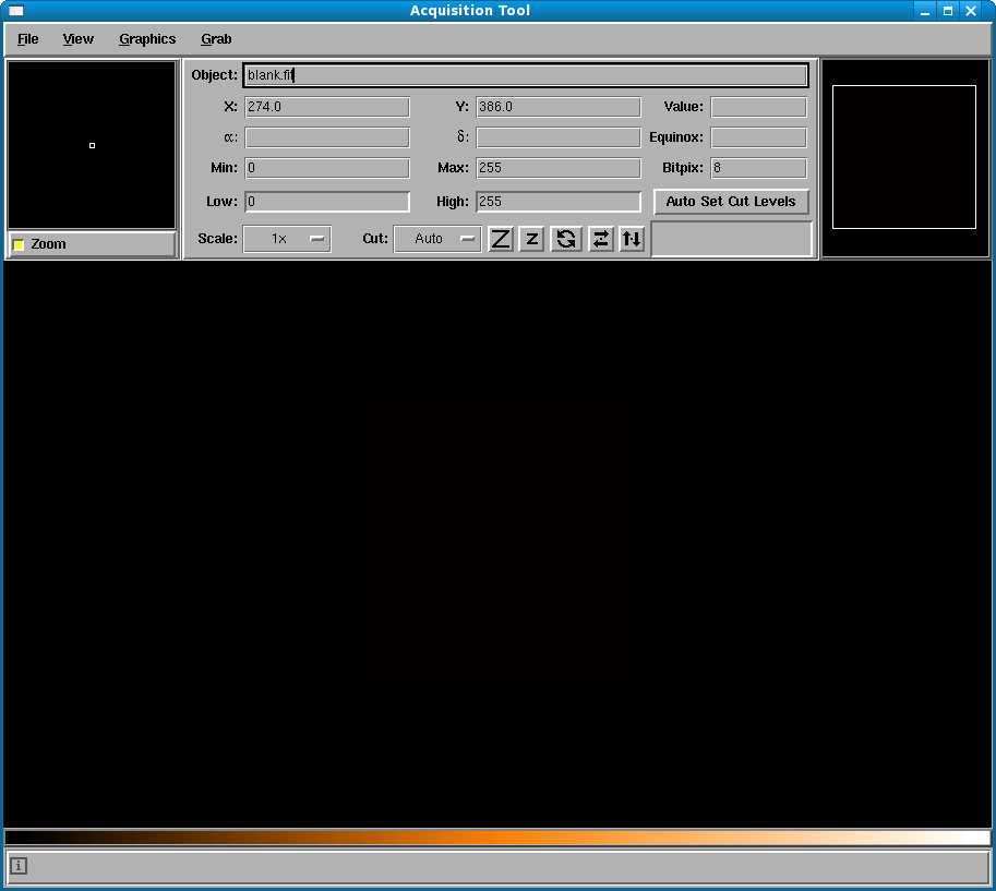
- The image below illustrates the main display page, which should appear when the tool is launched.
- Before using the acquisition tool, save the detector setup that will be used for the on-sky science observations:
SYS> saveccd
acam <user selected name>
E.g.
SYS> saveccd acam acam20100719
The acquisition tool will automatically change the ACAM detector setup [windowing, binning and read out speed] before taking an image grab and will reset the observer's setup afterwards. However should the acquisition tool crash, then the user may need to manually restore the detector setup.
6. Grabbing an acquisition image
- To bring up the ACAM Image Acquisition window, go
to
the
menu option Grab and select Grab ACAM Acquisition Image.
Alternatively
you can press Ctrl-a on the keyboard, while the mouse is
located over the main display page.
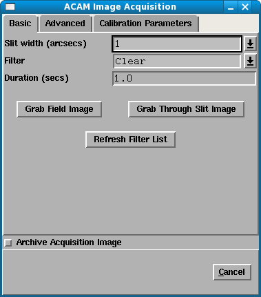
- The GUI has three tabs. The 'Basic'
and 'Advanced' tabs are used to grab the images, while the
'Calibration Parameters' tab can be used by the instrument
specialist or telescope operator to calibrate the acquisition tool.
More details on these interfaces are given in the subsections below.
- Before taking any grabs, make sure that the telescope is
configured for the 'Cassegrain' focal station.
The image below shows the 'Basic' grab GUI:
6.1.1 Grab Buttons
Both 'Grab' buttons will perform the following functions:
- Check that the CAGB mirrors are configured to the "agacam"
position and, if not, warn the user.
- Configure the ACAM mechanisms for imaging mode (either without or
with the slit deployed).
- Configure the camera server for (i) an appropriate windowing, (ii) 1x1 binning and (iii) fast readout speed.
- Take an ACAM integration.
- Display the image on the main acquisition tool GUI.
- Reconfigure the camera server to its original configuration.
- Grab Field Image: This
takes an exposure in normal imaging mode and displays the image with an
overlay of the slit position. This option can be used to (i) image the
central 4'x4' field to which the telescope is pointing, (ii) confirm
the orientation of the field with
respect to the detector, and (iii) identify the position of the science
target.
- Grab Through Slit Image:
This takes an exposure in imaging mode, but with a slit deployed into the light
path. An overlay of the slit is also drawn. This option can be
used to (i) confirm the position of the slit, (ii) redefine the slit
overlay, and/or (iii) check that the target is falling down the slit.
6.1.2 User Options
There are three parameters that the user can change:
Slit width
Options: 0.5, 0.75, 1, 1.5, 2, 10, Clear
The user should select the slit width (in arcsec) that they will use for the spectroscopic observations. The value will be used (i) to draw a slit overlay of the appropriate width on the grabbed image and (ii) to deploy the appropriate slit into the light path (for the 'Grab Through Slit Image' option). Note that the default value is "1". Remember that the different slits do not have their slit centres aligned. Don't place an object at the centre of one slit, and then perform spectroscopy with a different slit.
If the 'Clear' option is selected, no slit overlay will be drawn when grabbing a 'Field Image'. Note that if you attempt to use this option for grabbing a 'Through Slit Image' a warning message will appear saying "Unable to perform ACAM configuration change".
Filter
Options: Clear, Current Setup, <List of filters>
These options allow the user to select the filter through which the image grabs should be taken:
Clear: Both filter wheels will be positioned in the 'CLEAR' position.
Current Setup: The filter wheel positions will not be changed from their current positions. (This option is useful if you don't want the acquisition tool to move filter wheels. However the acquisition image will not be of use if there is a blank, a grism or two [mismatched] filters in the light path.)
<List of filters>: The menu will list in alphabetical order all the filters loaded in the instrument. Any blanks or grisms will be ignored.
Note that the default option is 'SloGunR' provided that it is mounted into ACAM. Otherwise the option will default to 'Clear'. (Aside: Once the new Sloan filters arrive then the new Sloan R filter should be made the default option.)
If you select a filter that is located in filter wheel 1, then filter wheel 2 will be moved to the clear position, and vice versa. Note that the drop down menu will also include any filters in the focal plane slots. These can be used with the 'Grab Field Image' option to perform an imaging acquisition. (In this case, both filter wheels will be set to the clear position.) However if you try to take a 'Through Slit' image there will be an error message, saying "Unable to perform ACAM configuration change" - this is because the focal plane filter and the slit cannot be deployed at the same time. Once you click on 'OK' the detector parameters will be reset to their original setup.
When selecting which filter option to use, bear in mind the following points:
1. It is best to acquire the target
using a filter of a comparable wavelength to the spectral wavelength
most of interest, particularly if you are not using the parallactic
angle and are observing at large airmass. Otherwise the effects of
atmospheric refraction may mean that the object is not well centred on
the slit.
2. Broad band filters are generally
best for fainter targets, while narrow band filters are useful for very
bright targets that would otherwise saturate the detector.
3. Narrow band filters that match the
emission wavelength of an object that has strong line emission may be
more appropriate than a broad band filter as they will reduce the sky
background.
4. Using white light (i.e. the clear
option) will allow more target photons to reach the detector but (i)
the sky background will also be larger and (ii) the target will be
elongated if observing at large airmass.
Remember that ACAM will automatically send differential focus offsets to the TCS whenever one or more of the mechanisms are moved.
Duration (secs)
The exposure time in seconds can be selected by editing the 'Duration' field. By default a value of 1s is selected.
Note that if you need to change or stop an integration after you have pressed one of the 'Grab' buttons, you can use the usual ultradas commands, e.g.:
> newtime acam 30 [Change the exposure time requested to 30s.]
> finish acam [Close the shutter and read out the detector straightaway.]
> abort acam [Kill the exposure but don't store the image.]
With the 'newtime' and the 'finish' commands, the exposure will be read out and displayed by the acquisition tool as normal.
If you use the 'abort' command you will receive a warning from the acquisition tool that the grab was not successful:
"Unable to perform integration on camera AUXCAM. IDL: UDAS Camera/Error Info:1.0{Info{Exposure aborted.}}"
Once you click on 'OK', the detector will be reconfigured to its original setup.
6.1.3 'Refresh Filters' button
The options given in the 'Filter' drop down menu are determined by an interrogation of the Filter Database when the acquisition tool is started. If you subsequently physically change the filters and update the filter database, then you need to refresh the list of options by clicking on 'Refresh Filters'. (Note that you can do this from either the 'Basic' or the 'Advanced' tab - the filter options are synced between the two tabs.) If you do not update the filter list then (i) you cannot use any of the new filters and (ii) you will get an error message when you try to use an old filters.
6.1.4 'Archive Acquisition Image' tick box
The 'Archive Acquisition Image' tick box allows the observer to select whether or not the acquisition images should be archived.
If archiving is selected:
- A scratch exposure will be taken.
- The exposure will be written to the file s3.fit.
- The exposure will then automatically be 'promoted' to the next available run number, rxxxxxxx.fit, and the file s3.fit will no longer exist.
- The run will be located in the usual /obsdata directory and the details of the exposure will appear in the observing log.
- The title of the run will be:
- AcqAF:<TCS catalogue name> (for 'field images')
- AcqAS:<TCS catalogue name> (for 'through slit images')
where the stem stands for 'Acquisition' with 'ACAM' while observing the 'Field' or the 'Slit'.
If archiving is not selected:
- The scratch exposure will be taken and written to s3.fit.
- The file will be overwritten the next time that an acqtool grab is taken.
- If you decide that you wish to keep the exposure (before it is overwritten) then you can manually promote the image from the pink ICS window using the following command: 'SYS > promote 3'. The exposure will appear in the /obsdata directory and the log.
6.2 ADVANCED ACQUISITION
The image below shows the 'Advanced' grab GUI:
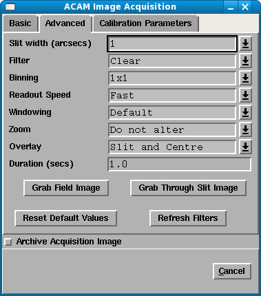
The basic functionality of the 'Advanced' mode is very similar to that of the 'Basic' one, with the same 'Grab Field Image' and 'Grab Through Slit Image' actions. However there a number of options one can use to modify the way in which the image is grabbed and displayed.
The 'Slit width', 'Filter' and 'Duration' parameters and the 'Refresh Filters' button will not be discussed further as they are described in the Basic Acquisition subsection. The other options are as follows:
Binning
Options: 1x1, 2x2
For 'Basic Acquisition' a 1x1 binning is used, giving a pixel scale of 0.25"/pixel. However in the 'Advanced' tab this can be overridden to give a 2x2 binning (i.e. 0.5"/pixel). This option may be useful when observing with one of the wider slits when (i) there are poorer seeing conditions or (ii) the target is extended. The advantages of using binning are (i) a higher S/N per pixel for the target in the same integration time and (ii) a faster readout of the detector.
As usual, the detector will be automatically configured before the exposure is taken and returned to its initial setup after the exposure has been read out.
Note that due to an as yet unresolved problem with the coordinate transformations, there can be slight shifts between the slit overlays in different coordinate systems. Please bear in mind:
1. All the 1x1 overlays are self-consistent with each other regardless of the windowing.
2. All the 2x2 overlays are self-consistent with each other regardless of the windowing, except for 'Full FOV'. Switching between the two standard windows (Slit window, Field window) with 2x2 binning should be no problem.
3. The 1x1 overlays are consistent with the 2x2 'Full FOV' window but not with the other 2x2 windows.
Therefore until this problem is fixed:
1. 1x1 binning can always be used safely.
2. 2x2 binning can be used but:
a) The 2x2 'Full
FOV' window is best avoided.
b) The 2x2 binning shouldn't be mixed with 1x1 binning. (Of course it is fine to switch binning when checking if the object is on the slit using a 'Through Slit Image', because one is not relying on the overlays.)
b) The 2x2 binning shouldn't be mixed with 1x1 binning. (Of course it is fine to switch binning when checking if the object is on the slit using a 'Through Slit Image', because one is not relying on the overlays.)
Readout Speed
Options: Fast, Slow
For a 'Basic Acquisition' the fast detector readout speed will always be used, while the 'Advanced' tab allows one to change the readout speed to slow. In general it is unlikely that you would want to use the slower readout as it will increase the acquisition overheads. However two possible situations where slow readout may be beneficial are:
- If you plan to also use the images for science.
- If there is a technical problem with the fast readout mode (e.g. excessive noise).
Windowing
Options: Default, Slit Window, Field Window, Full FOV, Unwindowed
One can select the windowing of the detector that should be used when grabbing an image:
Default: The windowing given by the 'Default' option (which as well as being the default value is also the windowing used by the 'Basic Acquisition' tab) depends on the type of grab being taken:
Grab Field Image: 'Field Window' (see below)
Grab Through Slit Image: 'Slit Window' (see below)
Slit Window: [325:1745,1885:1995] - A very small window is read out in the region where the slit falls. The region selected encompasses the full length of the slit and the height of the 10" slit (while including a slight border to cope with any flexure of the instrument). This windowing can be used with a 'Through Slit Image' for (i) identifying the position of the slit and/or (ii) ensuring that the target is falling down the slit. With 'Field Images' the small read out window can help speed up the finetuning of an acquisition, provided the object is close to the slit.
Field Window: [600:1550,1475:2425] - The chip is windowed to give a 4' x 4' field of view. This should be sufficient for most ACAM acquisitions to (i) identify the science target and (ii) place it on or near the slit. (For reference, the chip centre is y=2100, the slit centre is y~1950 and the derotator centre is y~1890.) The smaller FOV will speed up the readout time compared to reading out the full unvignetted 8' diameter FOV of ACAM. Note, however, that one does not see the full extent of the slit length - if you wish to place two objects at extreme positions on the slit then it is recommended to use the 'Full FOV' window.
Full FOV: [1:2148, 800:3300] - The chip is windowed so that only the non-vignetted part of the chip is read out. This windowing is identical to that recommended for ACAM science observations. This mode is useful for seeing the full imaging field of view of ACAM. It may be used (i) if the science target cannot be unambiguously identified using the 'Field window' or (ii) if you wish to place two objects at extreme positions along the slit length.
Unwindowed: [1:2148,1:4200] - The full 2148x4200 chip is read out. Note that rather than reading out the chip with all the readout windows disabled, instead a window encompassing the whole chip is defined. (It is implemented this way due to the way the coordinate system is defined when the chip is binned.) This mode is not expected to be used regularly on sky. However it is convenient for calibration purposes, because the calibration parameters use this coordinate system.
For both 'Basic' and 'Advanced' acquisition modes, the detector will be automatically configured before the exposure is taken and returned to its initial setup after the exposure has been read out.
Zoom
Options: Do not alter, Default, x1, x2, x3, x4
This options allows the user to select with what 'zoom factor' new image grabs will be displayed. The default value is 'Do not alter'. (This value is also used for the 'Basic Acquisition' tab). The options are as follows:
Do not alter: The current zoom that is selected on the main GUI will be preserved.
Default: The default zoom is selected for the particular type of image grab (i.e. 'Field image' or 'Through Slit image'). Currently a zoom of x1 is used for both types, however we may optimise these with experience.
x<n>: A zoom value of <n> is used, where n=1-4.
Overlay
Options: Slit and Centre, Slit, Centre, None
When grabbing a 'Basic Acquisition' image both (i) the slit overlay and (ii) the slit centre will be overlaid on the image. However in the advanced tab the user can configure which if any of the overlays should be shown:
Slit and Centre: Display both the slit outline and the slit centre.
Slit: Display only the slit outline.
Centre: Display only the slit centre.
None: Don't display the slit outline and slit centre. (Note that this option can be useful for an 'imaging acquisition'.)
The compass overlay will always be drawn.
Note that if you change this parameter then you can instanteaneously update the overlays shown on the image (regardless of whether the image was taken with the basic or advanced tab).
'Set Default Values' option
One can click on the 'Set Default Values' option to reset all the parameters back to their default values. (Note that the three parameters on the 'Basic' tab are synced, therefore they will also be reset.)
6.3 THE CAGB MIRROR CHECK
When you click on a 'Grab image' button, the acquisition tool will check whether the CAGB mirrors are configured in the 'agacam' position (also known as the LARGEFEED position) so that light from the sky reaches ACAM. If this is not the case, a pop up window will appear stating:
The ACAM mirror is not currently deployed. Please select the required action.
- Deploy ACAM mirror and take exposure
This option will configure the mirror
to direct the sky light to
ACAM
and carry out the usual 'Grab' procedures (see earlier this section).
Note that the mirror movement will take (i) ~19s when starting from the
'acamcal' mirror position and (ii) ~12s from the 'agmirror out'
position.
- Continue exposure with current setup
The
mirrors will be left in their current (incorrect) position, and the
usual 'Grab' procedures will be performed (see earlier this section).
Note
that this option will be useful while:
1. Testing that images can be grabbed from the camera server (e.g. during any afternoon checks).
2. Testing the acquisition tool while the CAGB mirrors cannot be moved for operational reasons.
3. Performing acquisition on-sky in the case that the mirrors are in the correct position, but their status is not being reported correctly (e.g. in an error state).
4. Crudely testing the slit alignment (using the calibration lamps), particularly if there is (i) a mechanism problem or (ii) ACAM has just been mounted.
- Abort exposure
The exposure will not be started and the ACAM/CAGB mechanisms will not
be moved. (The detector parameters will be reset to their original
settings.)
7. The Display and Manipulation of Acquisition Images
7.1 Displaying Acquisition Images
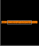
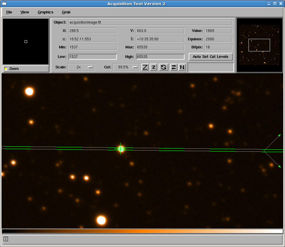
The acquisition tool will automatically display the images that it 'grabs' in the main GUI window, along with any overlays. An example of the display is shown below:
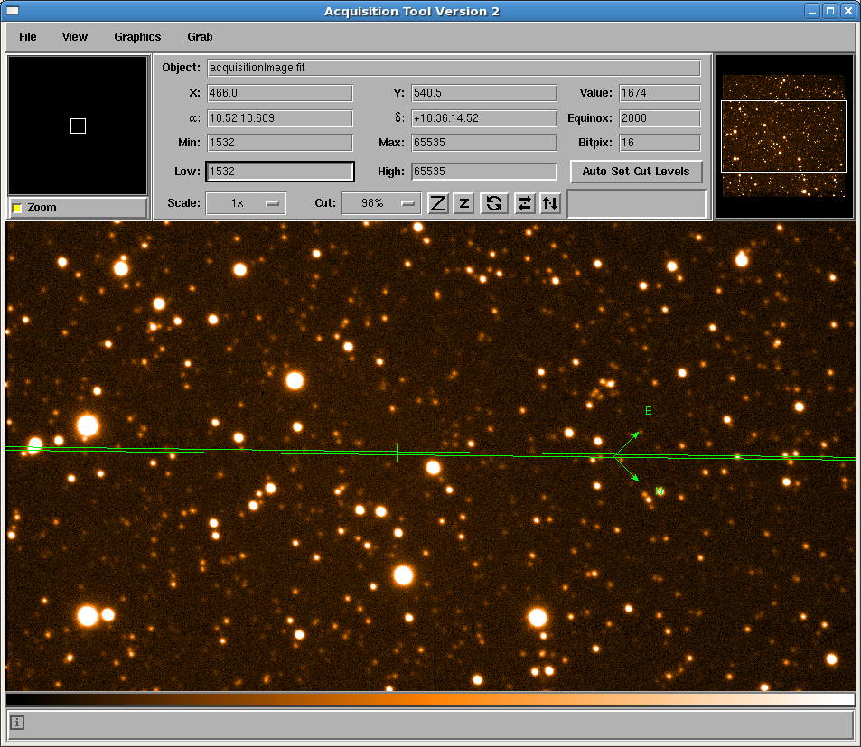
One can see the slit centre (cross), the slit outline (slightly tilted horizontal lines) and the compass.
The tool (i) applies the same 'cut levels' as previously selected from the drop down menu on the main GUI and (ii) attempts to conserve any flips or rotations that have previously been applied. (Unfortunately the orientation is not always preserved due to a bug in the underlying software.) The behaviour of the image 'zoom' is discussed here.
(Note that if the user has opted to archive the images then the exposure will be stored as a normal run in the /obsdata/whta/<date> directory. Otherwise the image is temporarily stored in the scratch file s3.fit and will be overwritten the next time an acquisition image is taken.)
7.2 Manipulating Acquisition Images
For those people familiar with this interface (e.g. skycat, GAIA, XOasis, other ING acquisition tools), most of the tools for manipulating images will be familiar. However there are a couple of minor differences. Most of the controls can be found in the top section of the main window:
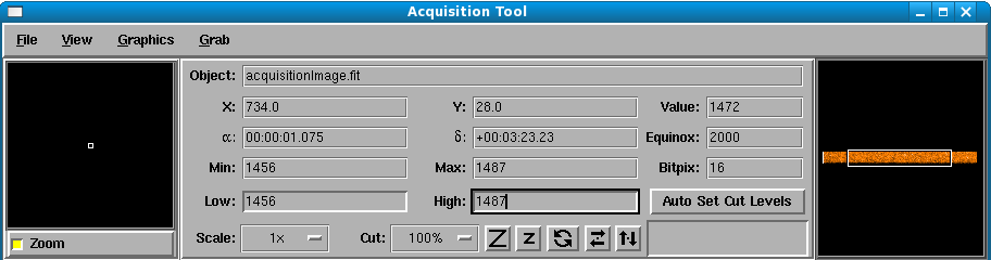
Display parameters
Firstly, there are various non-interactive display parameters:
X: The current x-position of the cursor.
Y: The current y-position of the cursor.
Value: The counts at the current position of the cursor.
α: The current right ascension.
δ: The current declination.
Equinox: The current equinox.
Min: The minimum counts in the image.
Max: The maximum counts in the image.
Bitpix: The bit depth of the image.
The WCS is computed using the (i) telescope position, (ii) 'sky PA' and 'Camera Mount Error', (iii) pixel scale, (iv) binning and (v) derotator centre. It will only be as accurate as (a) the derotator centre position and (b) the telescope pointing. For more details, see the discussion about the Derotator Centre in the 'Calibrating the Acquisition Tool' section.
Please note that the α and δ symbols are currently corrupted when displaying the tool using a VNC session (e.g. with the remote observing system).
Changing the Zoom
There are various ways to alter the image magnification:
- To select a specific magnification, go to the drop down menu entitled 'Scale' and select the value you require.
- To zoom in:
- Click on the 'Z' icon:

or
- Go to the 'Pan' window (at the top right of the main GUI) and click on the middle mouse button.
- To zoom out:
- Click on the 'z' icon:

or
- Go to the 'Pan' window and click on the right mouse button.
When displaying acquisition images, it is important to be able to easily control the image cuts. When the acquisition tool displays a new image, it will use the cut level that is selected in the 'Cut' drop down menu on the main GUI. There are two types of options in this menu:
- Numerical options, ranging from 90% to 100%.
- An 'auto' option, which uses a 'median filter'.
- Using the 'Cut' drop down menu on the main GUI to select a
different value. [Recommended]
- Using the 'Low' field or 'High' field on the main GUI to select a new lower or upper cut.
- Clicking on the 'Auto Set Cut Levels' button on the main GUI.
(Note that this has the same effect as selecting 'Auto' from the drop
down 'Cut' menu. However it is subtly different because this action
does not update the option selected in the 'Cut' drop down menu -
therefore the next time you grab an image the cuts may not be set to
'Auto'.)
- Go to the 'View' option at the top of the main GUI and select 'Cut Levels' from the drop down menu. This will launch a 'Cut Levels' GUI. The cuts can be changed by (i) changing the 'Low' or 'High' values, (ii) sliding the bars, (iii) choosing an 'Auto Set' options or (iv) using a 'Median Filter'. Note that for the first two options, you must press 'Set' before the change is implemented.
Flipping and/or Rotating an Image
The image (and its overlays) can be flipped or rotated using the following icons:


Note that the ACAM detector is set up with east 90 degrees anti-clockwise of north, therefore no flip is required compared to standard finding charts.
Moving around the field of view
To move around the field of view (when the image is zoomed in) there are two options:
- Go to the 'pan window', click (and hold down) the left mouse button inside the white box, and drag the white box to select the desired FOV.
- Go to the main image, click (and hold down) the middle mouse button, and drag the mouse to scroll the image.
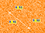
To measure the separation between two points, (i) go to the first point, (ii) click and (hold down) the right mouse button, and (iii) drag the mouse to the second point. A triangle will be displayed that is annotated with the x, y and total distance in arcseconds between the two points:
The Colour Map
There should be no need to adjust the colour map. If the image is not being displayed well, it is best to change the cut levels. However, should you wish to change the colour map, or more importantly reset it, this is how it is done:
- To shift the colour map, go to the 'Colourmap display' at the bottom of the main GUI, click (and hold) the left mouse button, and drag the mouse left or right.
- To reset the colour map, go to the 'Colourmap display', and click
with the right mouse button.

8. Redefining the Slit Position
8.1 The Uncertain Slit Position
The position of the slit centre must be accurately defined within the acquisition tool for the following reasons:
- The coordinates are used by the 'Move Object to Slit Centre' function (discussed in the next section).
- The acquisition tool displays overlays showing (i) the position of the slit centre and (ii) the extent and orientation of the slit.
- The slit centre will change with flexure (and therefore telescope elevation and derotator position).
- The different slits have different slit centres.
- Both the field image and the slit image are translated when you
change
filter.
- There may be other effects e.g. the positional reliability of (i) the slit mechanisms and (ii) the detector. (In practice the latter shouldn't be removed and remounted often.)
8.2 Defining a New Slit Centre
When performing a new acquisition, one should first check and if necessary redefine the slit centre. The procedure is as follows:
- Use the Grab Through Slit
Image function, making sure you select the correct slit. The
tool should display an image of the slit
and the overlays of the slit and slit centre. You may find it helpful
to change the image cuts.
- If the slit overlay is not coincident with the real slit, then bring up the Pick Object dialogue (see next section) and click on 'Select New Slit Centre Position'.
- Go to the image of the slit and click on the y-centre of the slit. (Note that this can be done at any point along the slit as the tool will compute the y-centre position at the true x-centre, after taking into account the slit rotation. On the other hand, to improve accuracy try to click somewhere near the x-centre, as opposed to near either end of the slit, unless this is where you are going to place your target.)
- Click on 'Apply New Slit
Centre' (in the Pick Object dialogue).
The slit overlay will be
redrawn. Check that it now accurately traces the real slit.
9. Acquiring Targets on the ACAM Slit
Once you have (i) checked that the slit position is accurately defined and (ii) identified the science target on an acquisition image, you are ready to acquire the target on the ACAM slit.
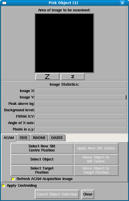
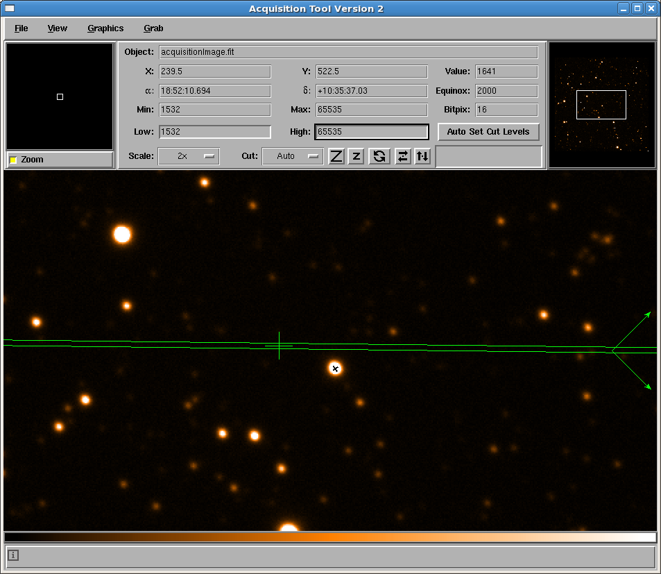
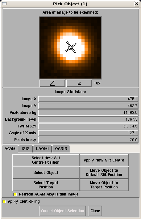
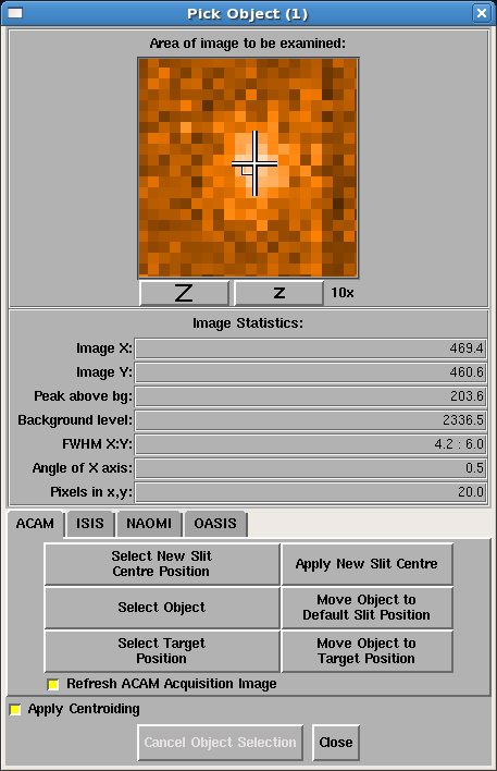
9.1 The Pick Object Dialogue
Science targets can be moved using the acquisition tool's 'Pick Object' dialogue:
- To bring up the Pick Object dialogue, go
to
the
menu option View and select Pick Object.
Alternatively
you can press Ctrl-p on the keyboard, while the mouse is
located over the main display page.
- The dialogue box has four tabs for (i) ACAM, (ii) ISIS, (iii) NAOMI and (iv) OASIS. By default the 'ACAM' tab should be selected.
There are two modes available for acquiring the science target: (i) Move Object to Slit Centre and (ii) Move Object to Target Position. For the majority of ACAM acquisitions (particularly those where you are placing a single target on the slit) option (i) is the recommended mode of operation for the following reasons:
- It is slightly more efficient as you only have to define one
position not two.
- The procedure is likely to be slightly more accurate.
- There is a smaller probability of user error.
- One will always place the targets at the same position on the
detector.
There are a couple of tick boxes that allow the user to slightly alter the behaviour of the Pick Object functions.
Refresh ACAM Acquisition Image: By default a new ACAM acquisition image will be taken after the telescope move has been applied. To prevent this, one can untick the box. (Note that a new image will not be taken if you simply redefine the slit centre position.)
Apply Centroiding: When one uses the 'Select Object' function (see below), a centroiding algorithm is applied to determine the object's position. While this normally works well, it may cause problems when selecting an extended target or an object in a dense field. In such cases, one can untick the box to (i) switch the centroiding off and (ii) use the exact position where one clicked.
9.3 Moving objects to the 'Slit Centre'
In this mode the user selects the science target and the acquisition tool moves the telescope to place the object at the 'Slit Centre'. This position is indicated by the cross shown on the image overlay. (The coordinates are also displayed in the 'Calibration Parameters' tab of the 'ACAM Image Acquisition' GUI - however in this case they are in the unwindowed and unbinned detector coordinate system.)
- Click on 'Select Object' in the Pick Object dialogue.
- Go to the main display window and click on the target that you wish to place on the slit.
- Check the image shown in the Pick
Object dialogue and confirm that the target has been correctly
selected.
- Click on 'Move Object to Slit Centre'.
- A TWEAK will be sent to the telescope.
- Once the telescope move is complete another ACAM exposure will be
taken using the parameters in the 'ACAM Image Acquisition' GUI (unless
the refresh has been disabled by the user).
- The image and overlay will be displayed.
In this mode the user selects (i) the science target and (ii) the position in the field where the target should be placed.
- Click on 'Select Object' in the Pick Object dialogue.
- Go to the main display window and click on the target that you wish to place on the slit.
- Check the image shown in the Pick Object dialogue and confirm that the target has been correctly selected.
- Click on 'Select Target Position'.
- Go to the main display window and click on the position where you
wish to place the target. For spectroscopy this will generally be at
the vertical centre of the slit; obviously one can select the
horizontal position
according to where one desires the target to fall on the detector.
(Note that one
could also use this mode for performing an imaging acquisition.) When
selecting a target position,
the
acquisition tool never
applies
the centroiding algorithm used for selecting objects.
- Click on 'Move Object to Target Position'.
9.5 Finetuning an Acquisition
For bright targets and/or wider slits, one may be able to use a single iteration to acquire a target on the slit. However for fainter targets and/or narrower slits, it is advisable to use a couple of iterations. The following strategy can be used:
1. Grab an acquisition image and use one of the Pick Object functions to move the target onto the slit while the telescope in tracking mode.
2. Start the guiding.
3. Take a new acquisition image. (Note that if you use the 'Advance' acquisition tab then you can use the smaller 'Slit Window' to speed up the readouts.)
4. If necessary finetune the target position using either (i) the Pick Object dialogue or (ii) a manual TWEAK. (If necessary you can use more than one iteration.)
5. Confirm that the target is correctly positioned.
6. Don't forget to switch to spectroscopic mode before starting the science exposure.
10. Example Acquisition Scenarios
The previous sections have given a detailed description of the different functions of the acquisition tool. The aim of this section is to give a coherent and visual overview of how to piece these functions together to perform an actual acquisition.
(Please note that there may be slight differences in the GUI labels due to minor updates. Also, in these examples, the slit is rotated by 0.68 degrees with respect to the detector because the image grabs were taken before the detector was rotated to improve the arc line alignment.)
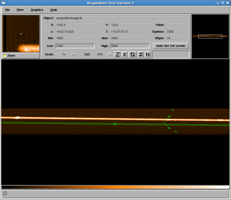
10.1 Scenario 1: Placing a single target on the centre of the slit
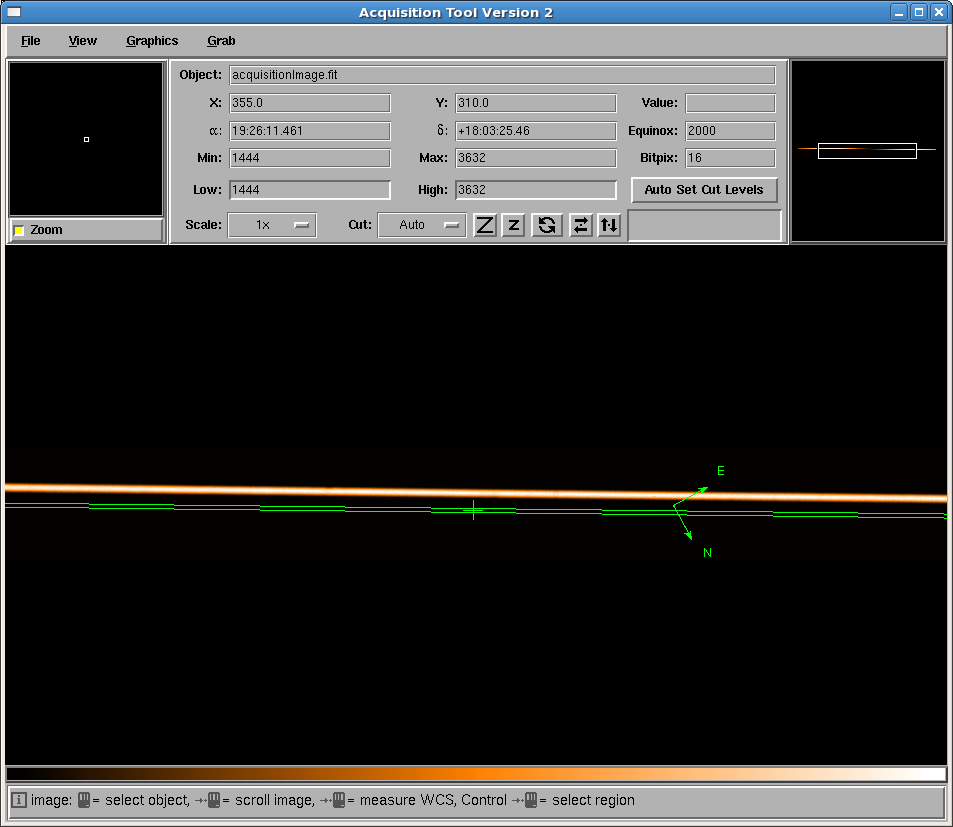
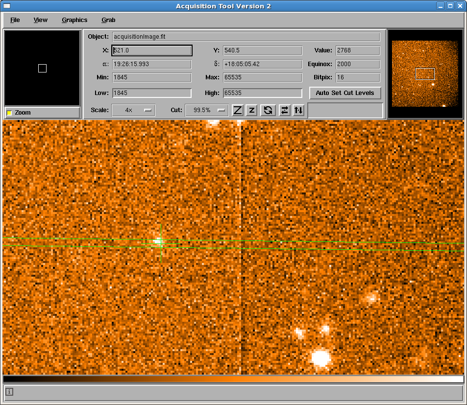
| 1. Move
to the new target (or ask the TO to do this) and wait until
both the telescope and the derotator are in TRACKING mode. Grab a
'Through Slit Image' (see §6)
to locate the position of the slit on the
detector. At this point the slit overlay may well be in the wrong
position, as shown below. |
|
 |
|
See an alternative example here. This field is much less dense and no objects fall on the slit. |
|
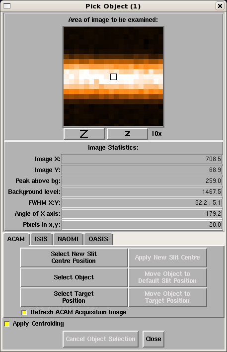
2. Use the 'Select New Slit Centre Position' function on the 'Pick Object' dialogue (see §8.2) to select the true position of the slit centre. |
|
 |
|
3. Use the 'Apply New Slit Centre' function (see §8.2) to apply the new slit centre. The overlay should now be correctly positioned over the slit image. |
|
 |
|
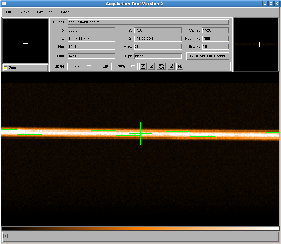
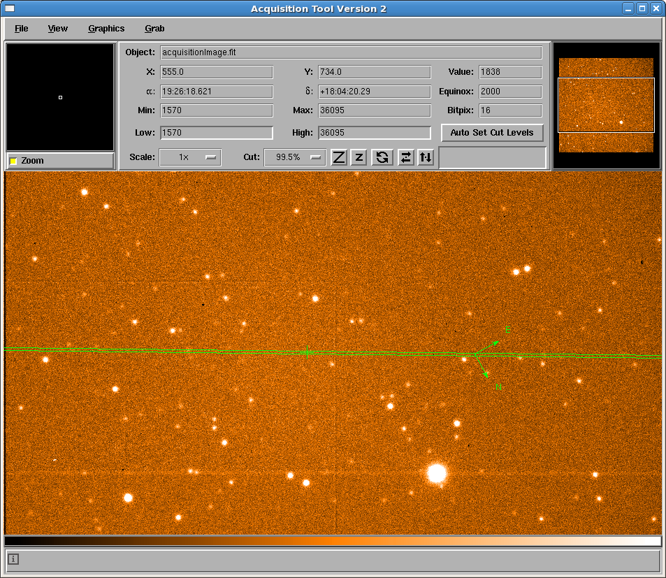
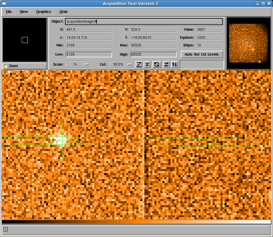
4. Grab a 'Field Image' (see §6) and identify the science target. |
|
|
|
See an alternative example here where a much fainter target is being acquired. |
|
5. Use the 'Select Object' function of the 'Pick Object' dialogue (see §9.3) to select the target. |
|
 |
|
See an alternative example here where a much fainter target is being acquired. |
|
6. The position and other properties of the target will be displayed in the 'Pick Object' dialogue. |
|
 |
|
See an alternative example here where a much fainter target is being acquired. |
|
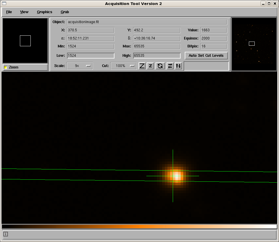
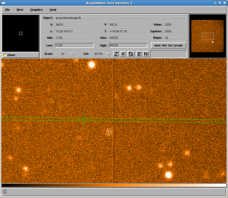
7. Use the 'Move Object to Slit Centre' function (see §9.3) to place the object on the slit. A new image will automatically be grabbed. The target should appear on or close to the slit centre. |
|
 |
|
See an alternative example here where a much fainter target is being acquired. |
|
8. Start the guiding and finetune the position of the target using the acquisition tool and/or the TCS handset (see §9.5). Note that the handset is better for very small sub-arcsec moves. The target should now be centred in the y direction of the slit overlay. |
|
 |
|
See an alternative example here where a much fainter target is being acquired. |
|
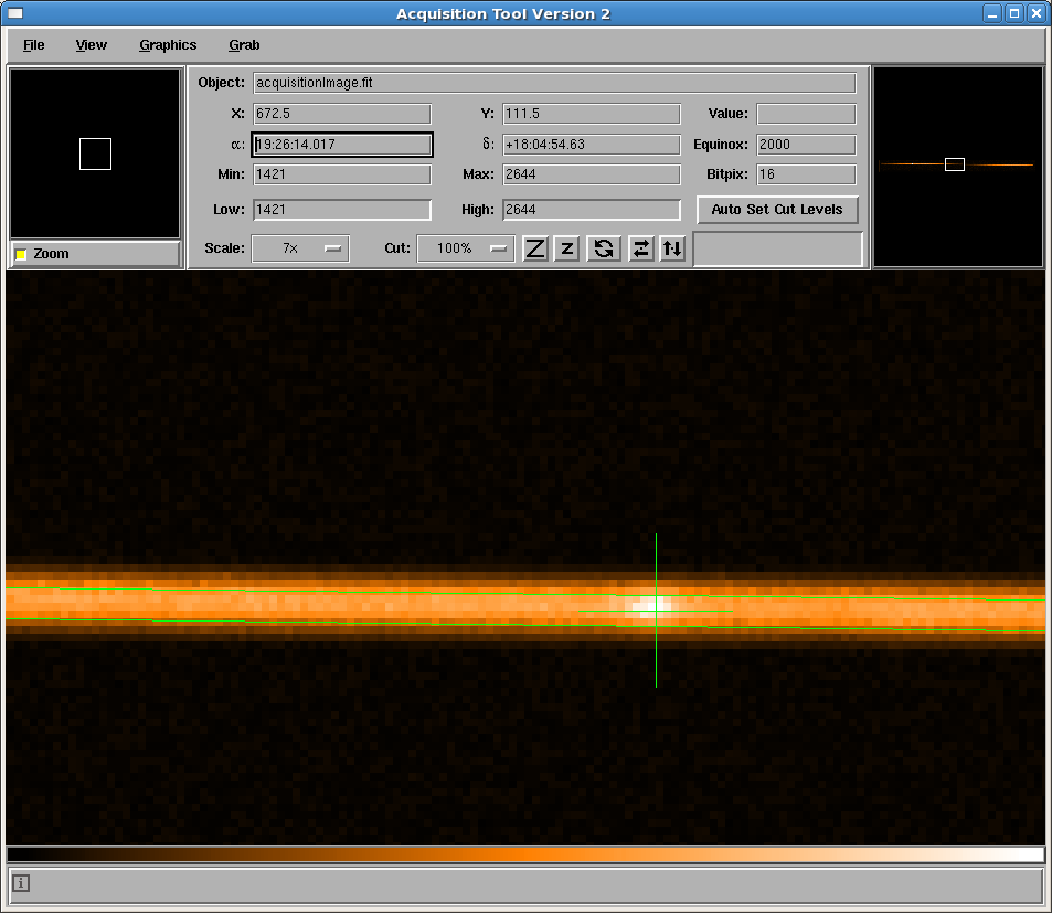
9. Grab a 'Through Slit Image' (see §6) to see an image of the slit and the target. Confirm that the target is well centred on the slit. |
|
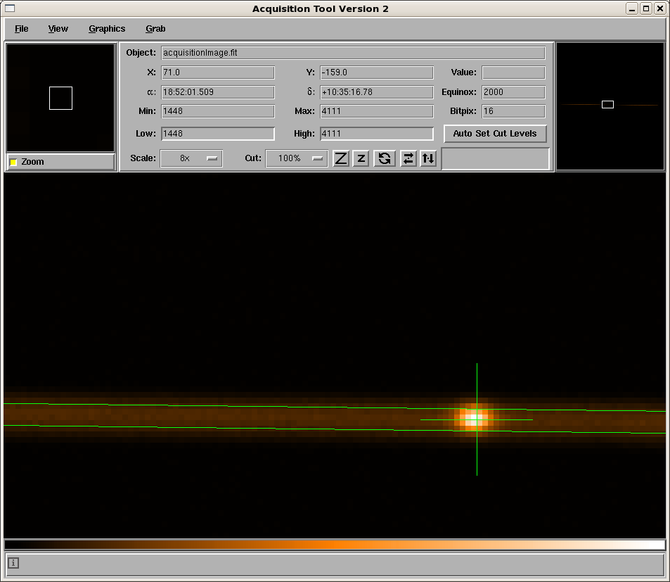 |
|
See an alternative example here where a much fainter target is being acquired. |
|
10. Configure ACAM for spectroscopy. This can be done from the command line using the following syntax:
|
|
| 11. Start the science exposure, e.g. TO> run acam 1800 "<Title>" . | |
More acquisition scenarios will be added in the future.
11. Checking the Telescope Focus
ACAM users should be aware that the telescope focus is automatically updated whenever you reconfigure ACAM for different filters or the grism. These updates occur regardless of whether you use (i) the GUI, (ii) the command line or (iii) the acquisition tool. The magnitude of the focus offset for each filter/grism is listed (and can be modified) on the 'ACAM Observer GUI'. The offset that is currently applied to the telescope can be seen on the 'TCS Display page'. The values shown are:
FOCUS <Focus demand selected using 'focus' command> TC <Value of temperature compensation> DF <Value of Filter Focus Correction>
These three values are used to compute the true focus to which the telescope should be set. Through the use of TC and DF, the user should never have to manually change telescope focus during the night. More general information about the focus offsets can be found in the ACAM Cookbook and, on the intranet, under (i) the ACAM Software Guide and (ii) the Filter Focus Offset Guidelines.
The important point is that you need to make sure that the telescope is focussed when ACAM is in spectroscopic mode (at the wavelength of interest). Ideally it should also be in focus when in imaging mode (with whatever filter is being used) so that the image quality of the acquisition images is good. It is important that users remember to check this - if the focus offsets are not found to be correct then they can be updated using the GUI.
12. Troubleshooting Advice
This section gives troubleshooting advice and will expanded if/when any problems arise. If you encounter any technical problems relating to the usage of the acquistion tool (including those issues discussed below) please (i) enter a fault report and/or (ii) notify Craige Bevil (cb@ing.iac.es).
11.1 Scenario 1: The tool crashes
- If the tool crashes, you can restart it manually as follows:
- Note that under normal operation, the tool automatically restores
the user's detector settings after each image grab. However this may not be the case if the tool has
crashed. If necessary, reinvoke the user settings (windowing, readout
speed, binning) that were stored earlier with the saveccd command:
SYS> acqtool&
SYS> setccd
acam <user selected name>
11.2 Scenario 2: The desktop freezes
- If the entire ICS desktop freezes, then you will need to kill the acquisition tool and restart it.
- Go to a different (unfrozen) desktop (e.g. whtdrpc1) and bring up a terminal.
- Log on to taurus as whtobs:
/home/whtguest> ssh whtobs@taurus
- Search for the process running the acquisition tool:
TO> ps -ef | grep acqtool
- Find the PID and kill the process:
TO> kill <PID>
- Confirm that the ICS desktop is now working.
- Follow the steps discussed in the Scenario 1: The tool crashes to restart the tool and reset the camera settings.
- If the image grab is not displayed and you receive the error
message 'Unable to find scratch file: /tmp/acquisitionImage.fit' then
this indicates a problem with the transfer of the image file to the
acquisition tool. This problem can occur for a few minutes after the
/obsdata/ date change, which takes place every morning at 10 UT.
- Try grabbing the image again. If this doesn't work, wait 5-10
minutes and try once more.
- If the problem cannot be resolved or occurs at any other time of day, please enter
a fault report or email Craige Bevil (cb@ing.iac.es).
13. Calibrating the Acquisition Tool (for Specialists)
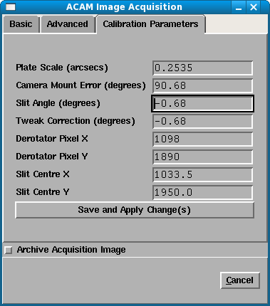
The acquisition tool will only function correctly and accurately if it has been well calibrated. The calibration values can be viewed and updated using the 'Calibration Parameters' tab of the 'ACAM Acquisition Image' GUI (see below). Note that updates to these parameters should only be made by trained instrument specialists or TOs.
A record of the calibration parameters has been created to (i) provide a reference point should the values be inadvertently changed and (ii) to keep track of any changes.
Please note that:
- The slit centre positions can either be changed (i) manually using this interface or (ii) automatically using the Apply New Slit Centre feature.
- All other parameters can only be changed manually using this interface.
- Nothing will happen unless you grab another image.
- The updated parameters will be used for all future image grabs
and any telescope moves.
- If the tool crashes, then the updated parameters will not be recovered. Instead the last saved values will be used.
- Some of the changes will be implemented immediately:
- If the 'Camera Mount Error' is updated then the compass will be
redrawn.
- If (i) the 'Plate Scale', (ii) 'Slit Angle' or (iii) the 'Slit centre' is updated then the slit overlay will be redrawn.
- The
WCS will not be updated after
a change to (i) 'Plate Scale', (ii) 'Camera Mount Error' or (iii)
'Derotator Centre', unless a new image grab is taken.
- The updated parameters will be used
for all future image grabs and telescope moves.
- If the tool crashes, then the updated
parameters will be restored.
Plate Scale
The plate scale (or pixel scale) is the size in arcseconds of one (unbinned) detector pixel. This parameter is used when computing the move that should be applied to the telescope in order to place the target either (i) at the slit centre or (ii) at the desired target position. It is also used for the WCS calibration. During the ACAM commissioning, Chris Benn determined x and y pixel scales of 0.253"/pix and 0.254"/pix respectively. Therefore, we are currently adopting a value of Plate Scale = 0.2535"/pix. This value should not be revised unless the instrument specialist remeasures a different value.
Camera Mount Error (degrees)
The 'Camera Mount Error' is used in conjunction with the telescope sky PA to calibrate (i) the compass that is overlain on the acquisition images and (ii) the WCS values. (It does not have any other effect on the operation of the acquisition tool.)
In January 2010, the TCS was reconfigured so that N would lie along the slit (pointing towards the right on an ACAM image) at a sky PA of zero. As the slit was rotated clockwise with respect to the detector rows by 0.68 degrees, a Camera Mount Angle of 90.68 degrees was used. On 10/11/2010 the detector was rotated so that the slit was better aligned with the detector rows, resulting in Camera Mount Error = 90.15 degrees.
Note that if the TCS is not accurately calibrated, then it is the TCS database that should be updated and not the acquisition tool. (On the other hand, if the slit is no longer at an angle of -0.15 degrees with respect to the detector, then the Camera Mount Error will need updating.)
Slit Angle (degrees)
The 'Slit Angle' defines the angle of the slit(s) relative to the rows of the detector. The same angle seems to be appropriate for all slits. This parameter is used when drawing the slit overlay on the acquisition images. (Note that slit overlays assume that the slits are straight, albeit rotated with respect to the detector - obviously any imperfections in the real slits will induce small differences between the overlay and the actual slit.)
When ACAM was first commissioned, the slit angle was -0.68 degrees. However since the detector was rotated (10/11/2010), Slit Angle = -0.15 degrees.
Tweak Correction (degrees)
It was decided for the purposes of spectroscopy that the TCS should be calibrated such that the x and y coordinate system of the 'TWEAK' command is aligned with the ACAM slit and not with the row and columns of the detector. (This was particularly important when the slit was poorly aligned with the rows of the detector.)
The 'Tweak Correction' defines the relative angle between the coordinates systems of the detector and the 'TWEAK' movements. This value is used by the acquisition tool when transforming the x, y shifts required on the detector to the x, y telescope tweaks required for the 'Move Object to Target Position' and 'Move Object to Slit Centre' functions.
Making the assumption that the TCS is accurately calibrated, a Tweak Correction = -0.15 degrees has been selected as this corresponds to the angle between the rows of the detector and the slit. (Prior to the detector rotation on 10/11/2010 this value was set to -0.68 degrees.) If the TCS is not accurately calibrated, then it would make more sense to update the TCS database than the acquisition tool.
(Note that in the future it might be possible to simplify the calibration parameters by combining the 'Slit Angle' and 'Tweak Correction'. However for the short term it was decided that it was safer to control these parameters separately.)
Derotator Pixel X and Derotator Pixel Y
The coordinates of the derotator centre are used to calibrate the WCS of the images. Note that they are defined in the coordinate system of an unwindowed and unbinned ACAM image. In October 2009, the centre was measured to be 1098, 1890 (which is to the right and down from the slit centre). In general the accuracy of the telescope pointing should be such that the target falls within 2" (and at most 5") of the derotator centre, therefore this is the accuracy to which the WCS will be defined. (If a higher degree of accuracy were required when examining a particular acquisition image then one would have to tweak these coordinates and grab another image.)
(Note that this value should be redetermined in the near future following the rotation of the detector on 10/11/2010.)
Slit Centre X
The 'Slit Centre X' parameter defines the x-position on the detector corresponding to the geometrical centre of the slit(s). This parameter has two purposes:
1. To define the x-position of the 'slit centre', which is used for (i) the 'Move Object to Slit Centre' function and (ii) the associated 'cross' overlay on the acquisition image.
2. To define the x-positioning of the slit overlay.
(Note that this parameter is used for two quite different functions - if for some reason it is found that is not desirable to place science targets at the geometrical x-centre of the slit, then the software could be upgraded so that there are two separate parameters.)
It is important to understand that the 'Slit Centre X' parameter is defined in the coordinate system of an unwindowed and unbinned ACAM image. When the user is using a different windowing/binning, the acquisition tool will take this in account when (i) computing the telescope moves and (ii) plotting the overlays.
Currently Slit Centre X = 1023.5. This value was determined using the 1" slit with the SloGunR filter and the telescope at zenith - if you use a different filter then shifts of ~5 pixels are possible. However as the exact position does not have to be extremely precise (unless one needs to see the overlay right at one end of the slit) the value of this parameter should not need to be altered. (Note that prior to the detector rotation that took place on 10/11/2010 the slit centre was 1033.5.)
Slit Centre Y
The 'Slit Centre Y' parameter is similar to the 'Slit Centre X' parameter albeit with important differences. It is defined as the y-position on the detector corresponding to the centre of the slit, at the x-position 'Slit Centre X' . (Remember that the slit is tilted with respect to the detector.) As for 'Slit Centre X', this parameter is defined in the unwindowed and unbinned coordinate system and has several purposes:
1. To define the y-position of the 'slit centre', which is used for (i) the 'Move Object to Slit Centre' function and (ii) the associated 'cross' overlay on the acquisition image.
2. To define the y-positioning of the slit overlay.
This position needs to be constantly refined because the slit centre will vary depending on several factors such as flexure and the slit/filter in use (see §8.1). There are two ways in which this value can be updated:
1. One can manually change the value in the GUI. In general this is not recommended - remember that the coordinate system is probably different from that of the acquisition image you are working with. Nevertheless this method could be useful if you want to manually tweak the centre by a couple of pixels or even a sub-pixel.
2. The recommended way to redefine this value is to use the 'Apply New Slit Centre' function. Note that after applying this action, the 'Calibration Parameters' GUI will automatically be updated with the new 'Slit Centre Y' value (after the value has automatically been converted to the unwindowed and unbinned coordinate system).
For reference, after the detector rotation (10/11/2010) Slit Centre Y = 1951 when you use a 1" slit with the SloGunR filter and the telescope at zenith.
Archive Acquisition Image
This tick box is discussed in the Basic Acquisition section.
14. Finally
For more information about the ING's acquisition tool please refer to the WHT Acquisition Tool User Guide. Any bugs/problems/suggestions relating to the usage of the acquisition tool should be sent to Chris Benn.
Version 1.0: Document created. (S. Rix, 29/10/2010).
Version 1.1: Updated troubleshooting advice. (S. Rix, 05/11/2010)
Version 1.2: Updated to reflect renaming of 'Move Object to Default Slit Position' to 'Move Object to Slit Centre'. Also revised the 'default' filter option in the 'Grab' drop down menu. (S. Rix, 17/11/2010)
Version 1.3: Added details of the 'Calibration Constants' web page. (S. Rix, 19/11/2010)
Version 1.4: Updated the section on the 'Calibration Constants' following the rotation of the ACAM detector. Also added some information regarding the binning option on the grab image interface. (S. Rix, 23/11/2010)
| Top | Back |
|
