If you plan to observe many targets, it's recommended to create
your own catalogue before your observing run for improved on-sky efficiency.
Please follow the instructions provided
The TCS requires proper motions to be entered in units of coordinate motion as seconds per year of right ascension and arcseconds per year of declination, together with the epoch of the coordinates.
For targets taken from Gaia DR2 note that (i) the coordinate system is ICRS, and (ii) the
epoch is 2015.5. The WHT TCS does not directly accept ICRS as a coordinate system description, so such coordinates
should be entered in the catalogue as equinox J2000 (the ICRS axes are consistent with the equator and equinox of J2000.0 to better than 0.1 arcsecond), for example,
J154859+341822 15 48 59.68 +34 18 22.3 J2000 -0.0027 0.048 2015.5
Differential tracking rates for fast-moving objects such as as comets should be given in units of coordinate motion as seconds per
second of right ascension and arcseconds per
second of declination. For such targets, an ephemeris listing positions with equinox and differential tracking rates, at UT epoch timesteps of five minutes spanning the UT date of observation, usually suffices for acquisition and tracking.
Back
to the top
2. The observing system and IRAF
2.1 Starting the
observing system
The observing system on taurus should
be started in the afternoon, and is usually already started prior to your run by
the operations team. It has four monitors, each with several windows:
- A pink, instrument control window (labelled WHTICS),
in which
commands for configuring the A&G box and instrument mechanisms, configuring the detectors and acquiring data are entered. The command-line prompt in this pink terminal window is currently SYS>.
- A window with the mimic display should be open
in the left monitor, which by
default usually shows a summary of the status of ISIS and the A&G box,
with a trace of
the
light path.
- Several xterm orange windows. These
terminals are for the DAS control of the cameras, and normally you do not need to
deal with them (it is better to iconify them).
- A proposal identification window. Your Support
Astronomer (SA) will have entered the PI's name
and proposal reference at the begining of the run, and these details are
written in the FITS headers of each image.
- The observing log. The log is
automatically updated each time a new file is written to disk. To add
comments on an entry click the relevant line, and this causes a dialogue box
to pop-up.
- Two detector status displays,
one for the blue and the other for the red arm. If more
cameras are operative, e.g., ACAM, similar displays will be
open for them. If you accidently kill a CCD status display, or can't locate it, a new one can be opened from the
global CCD status
tabbed window, which contains tabs for each individual CCD configured in the observing system, as well as a global summary listing of all.
- The talker window, which displays
a consolidated view of system messages.
- The instrument control GUI in which
you can configure the A&G box and ISIS setup. This is an alternative to doing so from
the command line in the pink ICS window described above.
- A TCS display window, which provides a useful overview of the telescope's high-level status. If this window isn't present type
tcsinfo& in the pink ICS window.
If something goes wrong with the system, e.g., it appears to "hang", ask for help
from your SA
or OSA (telescope operator). Also, instructions for starting up and shutting
down the observing system can be found
here.
2.2 Starting an IRAF data
reduction session
You can start an IRAF session on whticsdisplay1 for basic inspection
of images by opening a terminal window and running the commands:
- iraf (start IRAF)
-
ecl> cd
/obsdata/whta/'yyyymmdd' (change the working directory to the data-storage area)
- ecl> isis (initialise ISIS-specific local packages)
For more intensive tasks such as quick-look spectral extraction or data reduction, it's
recommended to log on to a dedicated Linux PC, such as
whtdrpc1, located
immediately to the right of the instrument control monitors:
- Username: whtguest
- Password: provided by your SA
- Open a terminal window
- Start IRAF as described above
If you plan to reduce your data on-the-fly please don't work directly on
images stored in the live
/obsdata/whta/'yyyymmdd' directory (which is cross-mounted
to
whtdrpc1). Instead, copy images
to a directory in the
/scratch filesystems, e.g.,
/scratch/whta/'yyyymmdd' or
/reduction/local/'yyyymmmdd', and
run your analyses on the duplicated data.
Back to the top
3. Common A&G box and ISIS mechanisms commands
3.1 The Mimic display
The status of ISIS is displayed in
the mimic window.
There are five selectable tabs in
this window; ISISP, ISISMechErrors, ISIS, ACAMINS and CAGBFilters.
Choose the ISIS tab to show an overview of the ISIS instrument
components and their status, as well as a schematic of the light path
through the instrument. The status flags are colour coded:
red means there is a problem,
blue means that a mechanism is
moving, and white means that a mechanism is healthy and in a previously demanded configuration.
3.2 Commonly used
A&G box and ISIS mechanisms commands
ISIS mechanisms can
be controlled from the WHTICS terminal window or
from the instrument-control GUI (next section).
WHTICS is a Linux
shell, so (1) commands can run in the background enabling multiple commands e.g., on the blue arm and red arm, to execute simultaneously, and (2) mechanism-control commands can be combined with
UltraDAS data acquisition commands as shell scripts to carry out sequences of procedures.
Consult the respective manuals for detailed descriptions of
A&G box and
ISIS
mechanisms' control.
The most frequent operations on mechanisms the
observer
will perform are listed and explained below.
To help visualise what these commands do
it's useful to refer to the ISIS layout
mimic.
1. Select which arm(s) to observe
with:
bfold 0
(to observe in the red arm only, i.e.,
dichroic slide out of the beam)
bfold 1 (to
observe in the blue arm only, i.e., dichroic slide fold mirror in the beam)
bfold 2
(to observe in both arms simultaneously, i.e., dichroic filter in the
beam)
Set the grating central wavelengths:
cenwave blue 4500 (set the
central wavelength in the blue arm to 4500Å)
cenwave red 6500 (sets the central wavelength in the red
arm to 6500Å)
2. Select the slit width:
slitarc 1.0 (sets the slit width to 1.0 arcsecond. The maximum slit width is 22.0
arcseconds, and the minimum slit width is 0.32 arcsecond.
Slit width temperature correction is implemented;
more details about this correction can be found
here.
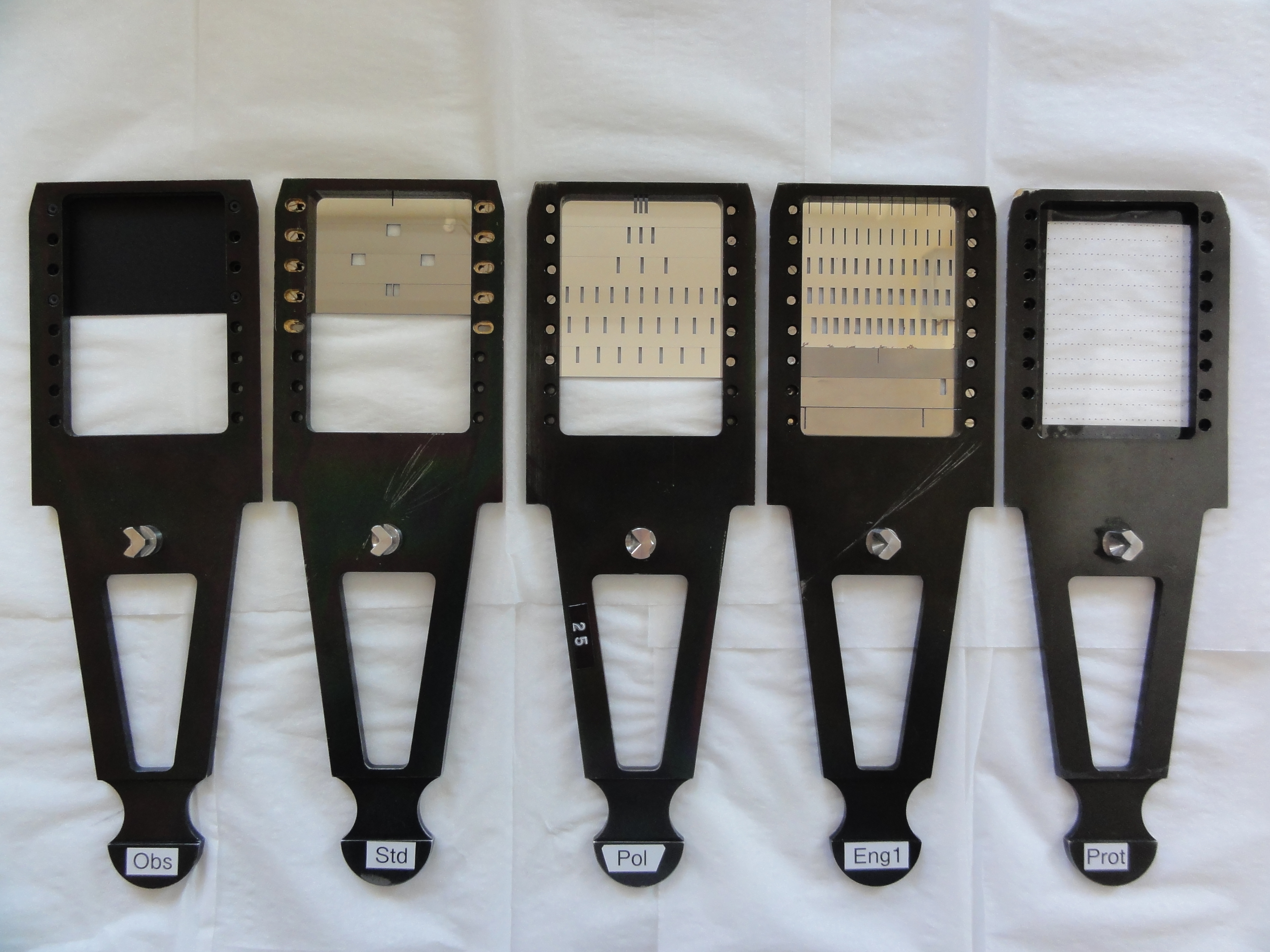
3. Select the dekker mask:
dekker 8 (set the dekker to the normal observing position, annoted as
CLEAR8 in the mimic).
The ISIS long slit module has a
slit
length of 4.0 arcminutes, of which 3.7 arcminutes is unvignetted. This is curtailed to
3.2 arcmin (blue arm) and 3.5 arcmin (red arm) when the default detector windows are set.
The dekker
slide is deployed above the slit to mask off the slit ends;
this reduces ghosting in ISIS and it's therefore strongly recommended
that
the dekker is deployed.
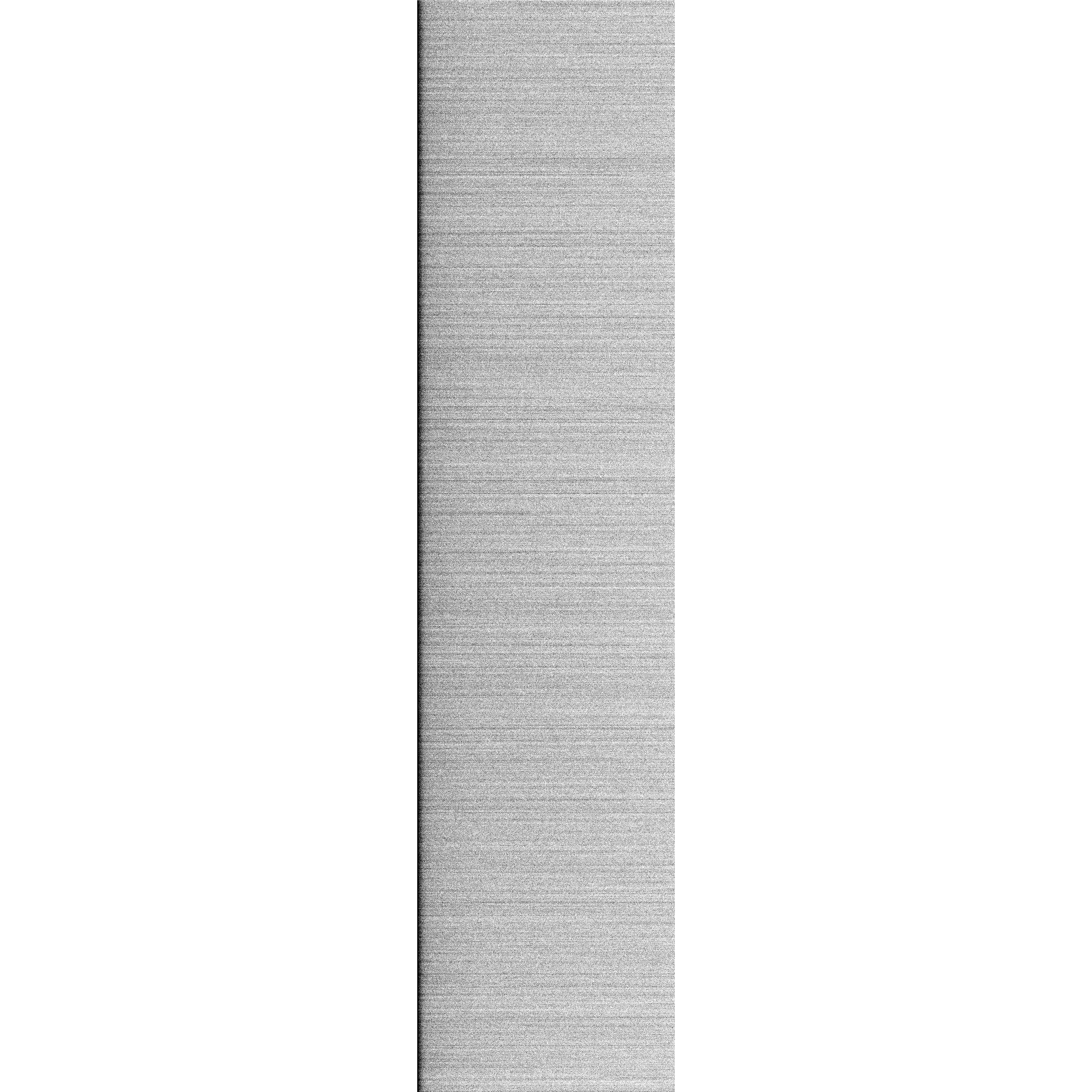
The available dekkers are shown in the photo. The default dekker used for long-slit mode (labelled Obs) is the one at the extreme left of this image.
4. Deploy a below-slit blocking filter in the red arm:
rfilta 3|1 (insert|remove the GG495 blocking filter in|from the beam after the red fold mirror)
Your support astronomer will advise if a blocking filter is needed to prevent
contamination of the red spectrum beyond ~6000Å by second order blue light. The
status of the below-slit filter slides is annotated in the mimic. Position 2 of rfilta contains an RG630 blocking filter.
5. Position the collimators at focus in each arm:
rcoll <red_focus> (red_focus is provided by your SA)
bcoll <blue_focus> (blue_focus is provided by your SA)
The spectrograph focus in each arm will be defined by your SA. However, if you have multiple
configurations such as different wavelength settings and/or different blocking filters in the
beam, you may have to reposition the collimators in each configuration.
6. Configure the slit to view the sky:
agslit (move the acquisition/comparison mirror out of the beam)
This moves the acquisition/mirror mirror in the A&G box out of the light path, so that light
from the sky falls on the slit. In this position the acquisition/comparison mirror directs light from the slit jaws to the acquisition TV, the
configuration which is shown in the mimic example. This command also turns calibration lamps off.
7. Configure the slit to view the calibration unit:
agcomp (move the acquisition/comparison mirror into
the light path)
This moves the acquisition/comparison mirror in the A&G box into the light path, so that light
from the calibration unit falls on its reverse side and is directed to the slit. In this configuration the acquisition TV cannot view the slit.
8. Turn calibration lamps on:
complamps w (turn the tungsten flat-field lamp on)
The available arc lamps are CuAr, CuNe and both together, CuAr+CuNe. Selecting
a different lamp turns the currently in-use lamp off, as does
complamps off and agslit.
Note: If you turn the lamps on first and then move the comparison mirror into the light path, the lamps are turned off when the agcomp command is issued.
9. Deploy a neutral density filter in the calibration unit:
compnd 0.8 (insert neutral density with attenuation of 0.8 dex)
The tungsten flat field lamp saturates the detector with low resolution gratings, and neutral density filters amelioriate this.
The calibration unit has two neutral density filter wheels, whose individual filter attenuations combine to reflect total demanded attenuation. The command compnd 0 removes the filters.
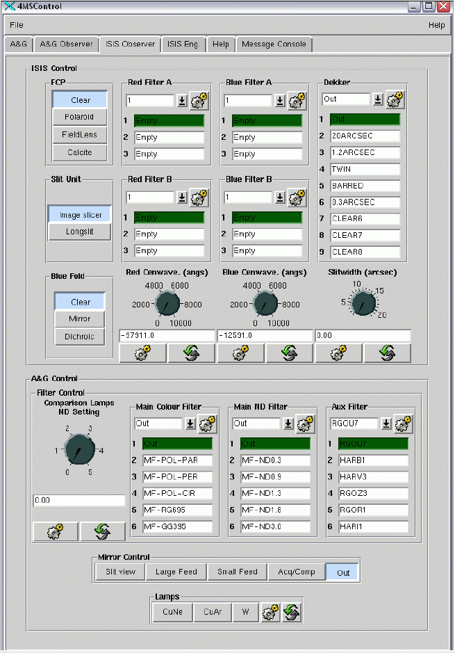
3.3 Controlling
A&G box and ISIS mechanisms from the GUI
The A&G box and ISIS mechanisms can also
be controlled from a
Graphical User Interface.
Manuals describing
the ISIS Control System and the A&G Control
System and use of the GUI can be found here
and here.
Using the GUI is very intuitive, and it suffices here to summarise the actions of their icons (see section 4.3 of the first manual linked above).
The GUI has several tabs; that most relevant to ISIS observing is shown here, and its icon semantics is summarised below
Back to the top
UltraDAS data acquisition commands
run in a Linux shell (
WHTICS), and so they can
execute in background mode by appending
& at the end of a given command.
This enables one to expose images simultaneously in the red and blue
arms. For example,
run red 900 & run blue 900 will take a 900s exposure in
each arm, returning the command-line prompt when the
blue-arm exposure
completes. Note that the exposure running in the background (red arm in this example) won't necessarily be complete
when the prompt is returned. Therefore, don't switch to calibration mode until exposures
in both arms are complete.
Ctrl+z followed by bg
suspends the current process running in the foreground and starts it running in the background. Therefore if you executed a pair of integrations as e.g., run red 900 & run blue 900; bell, so that the red-arm integration is running in the background and the blue-arm integration is running in the foreground (with an audio alarm queued to sound when the blue-arm integration completes in this instance), typing Ctrl_z then bg would cause the blue-arm integration to also run in the background, making the command line prompt available to issue, e.g., a pair of finish commands to the CCD controllers. Note that the bell command would execute immediately on typing Ctrl+z in this example.
As described in Section 3.2, UltraDAS commands can be combined with
A&G box and ISIS mechanisms commands to create scripts to execute observing sequences. Consult the
command dictionary of the UltraDas manual for a complete listing
and description of UltraDAS commands.
A summary of
the most frequently used data acquisition commands is listed and explained below.
Arguments to the commands are denoted by <>, and are (i) camera (red or blue),
(ii) integration time (s), and (iii) "title" (a descriptive title enclosed in quotes, stored in the FITS header).
If you do not specify a
title, the OBJECT name in the FITS header and in the nightlog will be the target name given in in your catalogue.
The run, flat and arc commands discussed all open the shutter
for the time specified, and differ only in the assignments to the OBJECT, OBSTYPE
and IMAGETYPE FITS header keywords. Similarly, images taken with the
bias command are identified as such in these FITS keywords.
- Set detector readout speeds:
rspeed <camera> <speed>
Sets the camera readout speed to slow or fast.
The operational characteristics for the two speeds are summarised for the EEV12 detector,
and for the Red+ detector.
Normally observations are carried out in slow mode because of the smaller read noise,
but of course for bright targets, especially where higher cadence is needed, fast
mode is preferred.
As noted, the default readout speed is fast on resetting the CCD controllers.
- Window the detectors:
window red 1 "[555:1520,1:4200]" (Set the default window on Red+)
window blue 1 "[585:1550,1:4200]" (Set the default window on EEV12)
The default windows on the Red+ and EEV12 detectors are 966 pixels wide, corresponding
to effective slit lengths of 3.54' and 3.22' respectively. The Y-axis window encompasses
the full detector extent, including the overscan region. Smaller windows of course can be
defined when high observing cadence is important.
- Bin the detectors:
bin <camera> <FX FY>
Sets the binning factors FX and FY in the spatial
and spectral directions respectively. For example, bin red 2 1 will
bin Red+ x2 in the spatial direction, leaving the spectral direction unbinned.
The spatial scales of the detectors are 0.20 arcsec/pixel (EEV12) and 0.22 arcsec/pixel (Red+). The grating dispersions and 1-arcsec resolution elements are
listed here for the EEV12 detector in the blue arm, and
here for the Red+ detector in the red arm.
It's not recommended to use 4x1 or 4x2 binning with the detectors windowed,
because the CCD controller times out and/or the observing system hangs
for a short time (due to internal error in the controller), and one or other of these occurs at least 50% of the time.
Also, high levels of binning are often accompanied by enhanced levels of clock-induced
charge.
- Save and recover detector configurations:
saveccd <camera> <filename> (Save detector configuration)
setccd <camera> <filename> (Recover detector configuration)
Saves the detector window, readout speed and binning to a named file, and resets the detector
configuration according to the named file description, respectively. If a filename isn't specified in
the saveccd and setccd command line, the default
filename udas_<camera>.cfg is used to store the configuration.
The setccd command is especially useful when a dasreset (next paragraph) has
been carried out, because the detector reverts to its default configuration following a reset.
- Reset the detector hardware and software:
dasreset <camera>
This is the first step to recover from persistent problems with the camera and controller. It resets
the detector hardware and software: (i) all processors in the SDSU
CCD controller are reset to their power-on state, (2) all processors
in the SDSU controller are reprogrammed, (3) the camera's configuration
including operating temperature is reloaded, and the detector geometry is
set to default values (no window and binning, fast readout speed). Unsaved
exposures are lost. The procedure takes typically 30s to complete.
- Take an exposure of a science target:
run <camera> <int time> <"title">
Takes an exposure of a science target and saves it as a FITS extension in rxxxxxxx.fit,
with the target identified in the FITS header keywords.
For example, run blue 600 "N157 B" take a 600s exposure
with the blue arm and write it to disk as e.g., r1826342.fit.
- Take multiple exposures of a science target:
multrun <camera> <n> <int time>
<"title">
Take n exposures of a science target and generates n distinct output FITS files (not n extensions to a single FITS file).
- Take an exposure of the flat-field calibration lamp:
flat <camera> <int time> <"title">
Takes an exposure of the flat-field lamp and identifies it as FLAT in the FITS header keywords.
- Take multiple exposures of the flat-field calibration lamp:
multflat <camera> <n> <int time>
<"title">
Takes n exposures of the flat-field lamp and generates n output FITS files.
- Take a twilight sky flat-field exposure:
sky <camera> <int time> <"title">
Takes an exposure of the twilight sky and identifies it as SKY in the FITS header keywords.
- Take multiple twilight sky flat-field exposures:
multsky <camera> <n> <int time>
<"title">
Takes n exposures of the twilight sky and generates n output FITS files.
- Take an exposure of the selected arc calibration lamp:
arc <camera> <int time> <"title">
Takes an exposure of the selected arc lamp and identifies it as ARC in the FITS header keywords
(the specific arc lamp selected is also identified in keyword CAGLAMPS).
- Take multiple exposures of the selected arc calibration lamp:
multarc <camera> <n> <int time>
<"title">
Takes n exposures of the selected arc calibration lamp and generates n output FITS files.
- Take a bias frame:
bias <camera> <"title">
Takes a zero-length dark frame and identifies it as BIAS in the FITS header keywords.
- Take multiple bias frames:
multbias <camera> <m> <"title">
Takes n zero-length dark frames and generates n output FITS files.
- Take a test exposure (of any type):
glance <camera> <int time>
Takes a test exposure in the current A&G box and ISIS configuration, and saves it to s1.fit.
This file is overwritten when the command is reissued. To convert a glance image to
a permanent copy type:
promote 1.fit (not promote s1.fit)
and it will be renamed to rxxxxxxx.fit by the observing system, where xxxxxxx is the next available run number in sequence. Do not simply rename s1.fit from the shell; the observing system would have no knowledge of this action, and the renamed file would be overwritten in the next invocation of an observing command.
- Take a scratch exposure (of any type):
scratch <camera> <k> < int time>
<"title">
Takes a scratch exposure in the current A&G box and ISIS configuration, and writes it to sk.fit, where k is an integer
in the range 1-99. In this way up to 99 test exposures can coexist. Of course subsequent
glance images would overwrite scratch file s1.fit, so it's wise to start scratch file numbering
at k=2.
promote k (rename scratch file k to the next available, permanent run number)
- Abort an exposure:
abort <camera>
Aborts an exposure which is running in the background without saving the data in the accumulated integration to disk.
- Stop an exposure early, saving the accumulated data:
finish <camera>
Terminates an exposure which is running in the background, and saves the accumulated data to disk. This is a useful
command when e.g., bad weather stops observing abruptly.
- Change the integration time of an exposure:
newtime <camera> <int time>
Changes the integration time of an exposure which is running in the background. For example, newtime red 900 would
change the integration time of the current red-arm exposure to 900s. This is a useful command when e.g., cloud cover thickens.
Back to the top
5. Afternoon checks and calibrations
In the afternoon before taking calibration images
it's wise to check the general configuration of the instrument and the detector readout speeds,
windowing and binning. These will have been set by your SA at the start of your run, but there's a small chance they may have been changed in the morning e.g., to troubleshoot a fault report, and not corrected.
Also, if the DAS has been reset to fix a problem, the detector windows will have been lost, the
readout speed will have been reset to fast and the detector will be unbinned. In this case windows, readout speeds and binning must be redefined as needed.
It's useful to take photographs of the instrument and detector mimics as a record of the configuration set up by your SA, so that you can refer to these on subsequent afternoons to check that the configuration remains as expected. If you fnd that an A&G box or ISIS mechanism, or a detector parameter, isn't configured as needed, use the appropriate command in Section 3 or Section 4 respectively to reconfigure it correctly.
Note that when the telescope is parked in "engineering mode", processed FITS headers such as
RA, Dec, parallactic angle and slit sky position angle in calibration images
are
incorrect. If the actual slit sky position angle is needed, e.g., for zenith spectropolarimetry
sky flats, it can be calculated from raw FITS header entries as described
here.
5.1 Taking calibration images
Before taking
calibration images turn off all dome lights (first check that nobody is working in the dome) and close the curtains in the
control room.
Flat-field exposures should not be brighter than approximately 40000 ADU to avoid issues with non-linearity of the detectors.
When using the low-dispersion gratings in the red arm the detector will saturate in short exposures of the tungsten lamp, so that neutral density should be deployed.
In the blue
arm arc exposure times in excess of 60s are needed to have well-exposed lines, and
it can be useful to take a much longer exposure (which will saturate these lines) to have some reasonably-well exposed lines in the bluest spectral region.
- View the calibration unit:
agcomp (moves the acquisition/comparison mirror into
the light path)
This moves the acquisition/comparison mirror in the A&G box into the light path, so that light
from the calibration unit falls on its reverse side and is directed to the slit. In this configuration the acquisition TV cannot view the slit, but can view the sky (with the X-direction opposite to that in slit-view mode).
- Turn calibration lamps on:
complamps <lamp> (turn the selected lamp on)
The available arc lamps are CuAr, CuNe and both together, CuAr+CuNe, and a tungsten lamp, w. Selecting
a different lamp turns the currently used lamp off, as does
complamps off and agslit.
- Take a test exposure:
glance <camera> <int time>
This exposure
will
allow you to compute a suitable exposure time to obtain well-exposed arcs or flat fields.
- If needed, deploy a neutral density filter in the calibration unit:
compnd <attenuation> (insert neutral density with attenuation in dex)
To remove the neutral density use compnd 0.
- Take lamp flat field exposures:
flat <camera> <int time> <title> (take a single flat-field exposure)
multflat <camera> <n> <int time> <title> (take n flat-field exposures
- Take arc lamp exposures:
arc <camera> <int time> <title> (take a single arc lamp exposure)
multarc <camera> <n> <int time> <title> (take n arc lamp exposures)
- Take bias frames:
bias <camera> <title> (take a single bias frame)
multflat <camera> <n> <title> (take n bias frames)
Before taking bias frames ensure that all the dome
lights and calibration lamps are off, and the blinds in the control room are closed. It's also
good practice to configure the comparison mirror in the beam (agcomp).
In principle, one can also take biases on ACAM simultaneously with those in the ISIS red and blue arms. However, it's been noted that taking
biases simultaneously for ACAM and the ISIS red arm causes additional noise in the form of horizontal lines on ACAM and the ISIS red arm,
which are not present if biases are taken separately. Taking biases on ACAM and ISIS simultaneously is therefore strongly discouraged.
- Take sky flats:
agslit (view the sky)
sky <camera> <int time> <title> (take a single sky flat-field exposure)
multsky <camera> <n> <int time> <title> (take n sky flat-field exposures
The internal-lamp flats, being free of lines, are of course used for
determining the CCD's pixel-to-pixel response. However, we suggest that observers take twilight sky flat fields to determine the slit
illumination function; knowledge of this is important
when observing extended targets or two (or more) point targets simultaneously in the
slit, and is useful for accurate sky subtraction.
To take sky flats with ISIS leave the
telescope parked at zenith in engineering mode (i.e., not tracking). In this way dithering between
individual exposures isn't needed.
For the higher resolution gratings (R1200R, R1200B, H2400B), you
should start ~10-15 minutes before a sunset, and for the lower resolution gratings
start around sunset.
Back to the top
6.1 Focusing the telescope
The focus applied to the telescope is
Fapplied = Fmeasured + dF(temperature) + dF(elevation) + dF(filter) mm
where the dF terms are corrections for telescope truss temperature, telescope elevation and filter focus offset. The temperature and elevation corrections are applied automatically by the TCS throughout the night to ensure the telescope remains focused on the slit as its environment changes. Example
values (in mm, taken from the FITS headers of image r2345903 on 20160412) are
Fmeasured = 97.85
dF(temperature) = 0.099
dF(elevation) = 0.055
dF(filter) = 0.00
Focusing the telescope in twilight therefore involves determining Fmeasured in the above expression. To do this, point to a bright star (r~9-11),
e.g., one of your
standards, at low airmass. It's usually fine to perform the focus run
in the default 1 arcsec slit, but if you prefer, you can open the slit
to e.g., 8 arcsecs, for the focus run:
slitarc 8.0
Since seeing is better at longer wavelengths it's preferable to focus using the
red arm, but it's wise at the start of your run to also check focus in the blue
arm, to ensure the best telescope focus is common to both arms.
Use fast readout speed to save on overheads, check that the detector isn't binned, and take a test image of ~10s to
check the level of the counts:
agslit (to view the sky)
rspeed <camera> fast
glance <camera> 10
The exposure time of the focus run needs to be ~7-10s to adequately
sample the
seeing. Inspect the test image to check that the spectrum isn't saturated and has SNR of at least ∼50 per pixel, and then execute the focusrun script:
focusrun <camera> <number exp> <int time> <focus start> <focus increment>
Typical parameters in an ISIS focus run are:
focusrun red 9 10 97.7 0.05
This will take nine images of 10s each, changing the focus of the
telescope from 97.70 mm in increments of 0.05 mm between the images.
All nine images are saved to path
/obsdata/whta/"yyyymmdd", and you can determine the best focus by analysing "manually" the
spatial profile in each image using
IRAF/imexamine. However, it's preferable to run the bespoke focus script
isis_focus directly
on the nine images in the
IRAF window at the
ecl prompt:
!isis_focus
Note that the preceding exclamation mark is necessary to escape the command (isis_focus is a Python script, executed at the Linux shell level).
The script prompts for the run number of the first image (without the ".fit" extension, e.g., r1234567)
and the number of images taken in the focus sequence.
The first image will then open in ds9 and you can position the cursor on the spectrum and press any key (e.g., spacebar)
to measure the spatial profile at that position. All subsequent images are displayed
one-by-one, and a spatial profile fit is
shown for each image in the sequence. Finally, a graphical window opens showing the measured
FWHM versus the telescope focus, with a parabolic fit
over-plotted. The best empirical and fitted telescope
focus values are printed in the IRAF terminal. Close this graphical
window to regain the ecl prompt in the IRAF session.
When the the best focus value has been determined
(e.g., 97.85) set the telescope to this focus and reset the detector readout speed to slow (if this is the preferred read speed):
focus <best focus>
rspeed <camera> slow
Warning: For runs involving both ISIS and ACAM, be aware that reconfiguring ACAM when ISIS is the selected instrument in use on-sky, will apply the configured ACAM optic focus offset, dF(filter),
immediately, defocusing ISIS immediately. If such a change were made to ACAM in the afternoon of an ISIS run, and an ISIS focus run performed in twilight with such a focus offset applied, the focus run will compensate for the focus offset. However, if the telescope focus is set to the ISIS nominal focus with such a focus offset applied, but an explicit focus run isn't performed (e.g. due to time constraints in twilight), the telescope will be defocused by an amount commensurate with the offset. In this case, if you notice that the dF parameter in the TCS window is non-zero, ask the OSA to remove it. Check at the start of the night that a focus offset isn't applied, and never change the configuration of ACAM while observing with ISIS.
Note also that the optimum telescope
focus, Fmeasured, is different for
ACAM and ISIS, distinct from any ACAM optic focus offsets applied, so care
is needed to ensure that the telescope focus remains optimal if switching
back-and-forth between these instruments. Reselecting ISIS after using ACAM
removes any ACAM optic focus offset applied, but otherwise does not change
the telescope focus to its ISIS value.
6.2 Target acquisition
Acquisition of targets in the slit will be carried out by the OSA.
Briefly, the slit jaws are polished and aluminised, and are inclined to the optical axis of the telescope at an angle of 7.5 degrees to allow the reflected image of the sky off the jaws
to be viewed by the A&G box TV camera, currently ag4. To configure the A&G box for acquisition and observing, issue the command
agslit
The TV camera images suffer from coma, and for "fainter" targets,
conservatively, V>18-18.5 dark-of-moon and V>16-16.5 bright-of-moon (and of course depending on seeing and extinction), blind-offset acquisitions are recommended (see Section 6.2.1 below).
The default orientation of the slit is set to the parallactic angle
at the mid-point of your integration by the OSA, but inform the telescope
operator if you prefer a different angle, for example, to place two targets in the slit, or to orientate the slit along features in an extended source.
Precession of the equinoxes causes a rotation of the equatorial coordinate
system (the direction of North changes), so if you plan to place two targets in the slit and therefore
need to orientate the slit along their common sky position angle, the
calculation
of this position
angle should be carried out in precessed coordinates, and of course where necessary, with coordinates corrected for proper motions.
This is especially true of very faint targets for which visual confirmation
of the acquisition may not be possible; for
bright targets the slit orientation can be easily adjusted to ensure
both targets are well centred. The impact of precession on sky position angle grows with declination.
To save an acquisition image, ask the telescope
operator to stop ag4 running in TV framing mode and execute the command
run ag4 <int time> <title>
This doesn't interfere with ongoing ISIS integrations, but remember to ask the telecope operator to switch ag4 back to TV framing mode, so that target centring in the slit can be monitored.
6.2.1 Blind offset acquisition
As noted above, the TV acquisition camera images suffer from coma, and for "fainter" targets,
conservatively, V>18-18.5 dark-of-moon and V>16-16.5 bright-of-moon (and of course depending on seeing and extinction) it's expedient
to first acquire a brighter object (brighter than the limiting magnitude)
close to the target (less than 20 arcminutes, but preferably less than
10 arcminutes from the target), and do a blind offset to your target.
In such cases prepare blind
offset stars in advance to save time. For accurate blind
offsets,
coordinates should be quoted to at least two decimal places
in seconds of RA and one decimal place in arcseconds of Dec. Always check if the offset
star has an appreciable proper motion.
Blind offset acquisition requires the coordinates of both the reference
star and the target, i.e., not coordinates of the reference star and
the offset distance to the target.
In the blind offset procedure, the accumulated
handset corrections applied to locate the reference object in the slit
from its initial "gocat" location
are converted
to tangent-plane coordinates, and these are added to the pointing model's
collimation terms in elevation and azimuth. This creates a localised,
incremental
correction to the pointing model, and this localised pointing model is adopted
in the blind offset procedure to position the faint target in the slit once
the reference target has been acquired accurately.
However, closing the loop on the reference star discards
this localised pointing model, and if the loop is subsquently opened and
a blind_offset applied, the rms offset accuracy will be degraded to at least 0.5-arcsec.
A blind offset should not be executed if the loop has been closed
on the reference object. For example, if a bright target in a galaxy or cluster is observed
closed-loop, then followed immediately by a blind offset to a faint target
in the same galaxy or cluster, the acquisition of the faint target will be compromised.
The procedure for making a blind offset acquisition is:
(i) gocat "target" and identify a suitable guide star
(ii) gocat "reference"
(iii) centre the reference object
(iv) quickly apply blind_offset "target"
(v) quickly close the loop
The rms accuracy of this procedure is <~0.2-arcsec. Open-loop
tracking error (~0.1-arcsec/minute) in the acquisition is minimised by
identifying
a guide star in advance of the blind offset, allowing the loop to be
closed quickly after the blind offset to the target completes, and of
course by quickly applying the blind offset once the reference target
has been centred in the slit.
It's good practice to take a deep exposure of at least 100s on the slit-view
camera following a blind offset acquisition to check centring of the target, e.g.,
accrued proper motion error could restrict acquisition accuracy.
Occasionally, blind offsets are needed to acquire a faint moving
target. In this case follow the above procedures and apply the blind
offset to the moving target less than one minute before the precise epoch adopted for the target coordinates, to limit open-loop tracking error. Apply the target's differential rates
at exactly the epoch of its coordinates; the target will ''drift'' into
the slit until the rates are applied, and the telescope will track it once the rates are applied. Close the loop immediately on applying the differential rates, and take a deep exposure on the TV to confirm acquisition.
6.3 Taking spectra of a target
First select the slit mode and slit width
agslit (view the sky)
slitarc 1.0 (set the slit width to e.g., 1-arcsec)
Ask the OSA to point to your target (it's useful
to provide a
catalogue of
the targets and their coordinates, and proper motions if relevant).
Also state the position angle you
want for the slit.
The OSA will take an image of the slit on the TV
camera, and when you've identified your target, will centre it in the slit and start
autoguiding.
When the OSA confirms your target is acquired and the telescope guide loop is closed, you
can start your integration by typing:
run red <exp_time> "<comment>" &
run blue <exp_time> "<comment>"; bell
An audio alarm will sound when the blue-arm exposure completes, in this example.
If you will observe with the slit at parallactic angle
(i.e. oriented in the vertical direction to minimise differential slit losses
due to differential chromatic refraction), it's advisable to adjust this at least every 1.5-2 hours because
the slit of course doesn't actively track the parallactic angle. The change
of parallactic angle with time can be determined using the
Staralt software
(select Option=Parallactic Angle).
Note that it's as important to adjust the
slit orientation every ~1.5-2 hours near zenith as it is at higher air mass;
although differential chromatic refraction is smaller near zenith, the rate
of change of parallactic angle is higher. These two effects combine to
make the relative movement of blue and red images across the slit only
weakly dependent on air mass.
If you do change the slit position angle to better track the vertical, always check the acquisition, and re-centre as necessary.
In the case of a target acquired in a blind offset, repeat the blind offset acquisition if you
change the slit orientation.
6.4 On-sky calibrations
To take arc calibration spectra (or lamp flats)
during the night, proceed exactly as described in section
5.2. for afternoon calibrations. Observers requiring accurate radial velocities should take frequent arc lamp calibration exposures,
e.g. every 15-20 minutes or so, to limit the impact of instrument flexure on radial velocity.
6.5 Observing bright targets
If you need to observe bright targets you can deploy the main neutral density
filters in the light path, so that light reaching each arm is attenuated. Take into
account that these neutral density filters are not uniform spectrally in the peripheral
regions of the detectors. The table below indicates the area of the chip in pixels
where the filters were determined to be "grey".
In addition to their spectral non-uniformity, all these filters have
small-scale throughput structures, which are
difficult to remove fully by flat-field correction. If there is a need to use these
filters (you should first consider narrowing the slit and/or defocusing the telescope as a solution in suitable cases), flat-fields should be taken to mask out affected regions.
To insert a main neutral density filter, use the command:
mainfiltnd <filter_pos>
where filter_pos is the filter position, corresponding to the
required attenuation in dex, as listed in the
table below. As an example, filter_pos 3 would correspond to an
attenuation of 0.9 dex.
The options are:
| Filter Position |
ND (dex) |
Useful Window |
| 1 |
0 |
- |
| 2 |
0.3 |
[500:1600,1400:2800] |
| 3 |
0.9 |
[500:1600,1900:3000] |
| 4 |
1.3 |
[600:1600,1400:3000] |
| 5 |
1.8 |
[500:1600,1400:2800] |
| 6 |
3.0 |
[1050:1550,1900:3000] |
6.6 Quick-look spectrum extraction
A basic quick-look spectral-extraction tool is available. We suggest that
you first copy data to be analysed to a scratch area,
e.g., /scratch/whta/'yyyymmdd' on the whtdrpc1 data reduction
computer.
To run the tool first
ensure the necessary IRAF local packages are initialised
(Section 2.2):
ecl> ing
ecl> isis
then at the isis> prompt type
isis> isis_ql <image number> <trace_X_pos>
where the image number is given without the '.fit' extension, and trace_X_pos
is the approximate X-position of the spectral trace on the detector.
For example,
isis> isis_ql r1234567 450
The script carries out an optimal extraction
(which takes about a second), and displays the spectrum in the IRAF graphics window using
splot. No wavelength calibration
is provided.
The usual splot keystrokes are available; for example, to zoom in on
a feature type w to enter window mode, position the cursor at the
lower left corner of the window you want and type e, and repeat this
at its upper right corner. Type w n to unset the zoom in flux,
w m to unset the zoom in wavelength, w a to unset the zoom in both axes, and q to exit splot.
Note that if the detector is binned, e.g., x2, in the dispersion direction, isis_ql still plots the extracted spectrum in unbinned pixels. Therefore a line expected to fall e.g., 300 binned pixels redward of the central pixel will fall 600 plotted pixels redward of the central pixel.
Back to the top
You can copy your data to location
laptop_path on your laptop when it's connected to the
ingext-WiFi or wired networks (ask your SA or OSA for the relevant passwords):
- rsync -avuz whtguest@whtdrpc1.ing.iac.es:/obsdata/whta/yyyymmdd/ <laptop_path>
Or,
you can copy the data to the FTP area, and subsequently retrieve it over the Internet:
- follow these
instructions:
Or, you can
write your data to a DVD (capacity ~4GB):
- ask your SA or OSA for blank DVDs
- follow these instructions


