 | |||
|

| Home > Astronomy > LIRIS > |
LIRIS Detector
Overview Table of Properties Windowing and Maximum Frame Rate Scrambled Pixel Mapping Bright Sources and Ghosts Bright Sources and Remanence Detector Reset Anomaly Flaws Exposure Times OverviewThe LIRIS detector is a 1024x1024 HgCdTe HAWAII array, manufactured by Rockwell Scientific Corporation. The main characteristics and features of the LIRIS detector are summarized below. More detailed descriptions can be found at the ING detector page and in the IAC report. IR detectors are very different from CCDs used in optical astronomy. For example, they show no blooming effects, and the same image can be read out several times (multiple non-destructive read mode, MNDR) in order to reduce the readout noise (this is useful for spectroscopy).LIRIS detector properties
(Top of page) Detector windowing and maximum frame rateUp to four non-overlapping windows can be specified for the LIRIS detector. The resulting image is as big as the unwindowed data, showing the windowed sections in their proper locations. Thus, unwindowed flatfields can still be applied correctly. Windowing is not recommended due to hardware limitations and since it usually leads to confusion during data reduction.To define a window, type in the pink observing system window: SYS> window liris n ``[ xmin : xmax , ymin : ymax ]'' enable or once it has been defined, you can disable it with: SYS> window liris n disable and also re-enable it later with: SYS> window liris n enable where n is the number of the corresponding window: 1,2,3 or 4. Windowing makes sense only if a source has to be covered with high time resolution. However, the efficiency gain is much less than expected, as shown in the table here. By using a window as small as 64 x 64 pixels and the shortest possible exposure time of 0.8s, a factor of only 2.3 can be gained as compared to a full-frame read-out.
(Top of page) Scrambled pixel mappingDue to some issues which are not explained further here, some of the pixels in the LIRIS image are not in the places where they should be. At some point in the digitisation process, the LIRIS data is in the form of a one-dimensional array, and part of this array is shifted by one index. When the two-dimensional image gets reconstructed, some of the pixels get dislocated. In particular, this affects the lower left quadrant, which is entirely shifted by one pixel to the right (easily recognisable in an arc image and in the sky lines of long-slit spectra). Its rightmost column gets wrapped around and appears on the left edge. A few isolated pixels in th other read-out quadrants are also dislocated. When you use the theli reduction package, all LIRIS images get automatically descrambled.(Top of page) Very Bright Sources and reflected ghost imagesWhen doing spectroscopy of very bright sources (and sometimes in flat fields), a ghost image of the source (or slitlet) appears on the detector, reflected around the centre of the chip (i.e. the optical axis). This has been noticed mainly in MOS spectroscopy, but also in long-slit spectroscopy. Hopefully, due to these ghosts being reflected around the centre of the detector, their location can be predicted by a script and accounted for during data reduction.Very bright sources and detector remanenceVery bright sources will leave a ghost image imprinted on subsequent exposures, which becomes visible when a dither offset has been applied in between. A default of 3 clearing reads is automatically applied before a new exposure is taken, which lowers the amplitude of the ghost to about 0.1-0.2% of the brightness of the original source. If this is still too much, you can increase the number of clearing reads to "n" bySYS> clearreads LIRIS n Using values of 6 or larger for n should largely eliminate the ghosting, for the expense of an increased overhead (2s for n=6). This holds for imaging and spectroscopy. (Top of page) Detector reset anomalyNear-IR detectors have very different properties from the CCDs used in optical instruments. While they are not being exposed, they are continuously reset and rapidly reach a resetting equilibrium. On the other hand, when a series of exposures is made, the detector reaches an imaging equilibrium. In an ideal world, there is no difference between these two states. In the real world, it takes about three exposures to go from the resetting equilibrium to the exposure equilibrium. This is recognised in a varying sky background that stabilises for the rest of the exposure series.However, even after the sky backgrounds have been calculated and subtracted correspondingly, there is an unstable component which shows up as a discontinuous jump between the upper and lower two read-out quadrants: 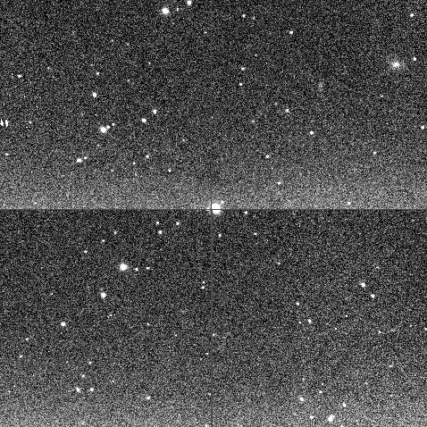 The amplitude of this jump depends on exposure time and illumination level, amongst other things, and the order of the image in a series of continuous exposures. There is also a large erratic component involved, hence this discontinuity cannot be modelled as a function of the parameters mentioned. Each image has to be corrected for this effect individually. Since the effect is also present in flat fields, the photometry of objects in the corresponding regions can be affected by 5-20%. The reset anomaly for LIRIS, after subtraction of an average sky background model. The amplitude and sign of the discontinuous jump seen varies from exposure to exposure. It is usually less pronounced than in this example, and often absent after sky subtraction. It can be corrected for by collapsing the images along their x-axis, using outlier rejection, and subtracting the average profile from each column. If you have dithered observations (see Imaging Scripts) and you take a series of e.g. 10 exposures per dither point, then the detector reaches the imaging equilibrium with the third exposure. All subsequent images will have the same image background as this third exposure. When you then move the telescope to the next dither point, the detector is reset during the slew and goes into the resetting equilibrium again and thus is in the same state as just before the first exposure sequence. Therefore, the image backgrounds are the same for the i-th exposures in the n-th sequence. The consequence is that the sky background has to be determined separately for each group of images. Example: You have 12 images per dither point, and you know that the detector settled into its equilibrium with the third exposure. Then you need to calculate three different sky backgrounds. The first is for the group of images 1, 13, 25 etc in the entire obseving series. Images 2, 14, 26 etc form the second group. All the remaining images have the same sky background and form the third group. After the three sky models have been subtracted from their corresponding images, the exposures can be merged again and treated together for the remaining reduction steps. See also *** theli_cal and *** theli_sf for how to do that with the theli software package. Please note that a certain fraction of images in the first group, which suffers most from the reset anomaly (and the poorer temporal sampling), can still have bad image backgrounds after sky subtraction. These images should be discarded. When you plan your observing strategy, take this into account and increase e.g. the number of exposures (nruns) taken per dither point by one. (Top of page) Detector FlawsThe LIRIS detector has a number of cosmetic features. Most noticeabe are:
Individual exposure timesThe individual exposure times are difficult to estimate. Most observers want to stay below 20-25 kADU for their science target in order be in the linear regime (<2% nonlinearity) of the detector: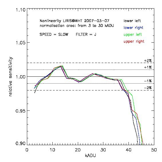 This of course depends on the sky background, dust level and extinction, and the current seeing. The individual integration times are therefore best determined by means of test exposures just before the actual observations. IMPORTANT: the readout noise value given in the image FITS headers is fixed, and regularly updated, but not derived from each individual image. Observers are therefore recommended to check the readout noise of their images. | ||||||||||||||||||||||||||||||||||||||||||||||||||
| Top | Back |
|