 | |||
|

| Home > Astronomy > ISIS > Spectropolarimetry user guide |

|


ISIS spectropolarimetry user guide
It's usually recommended to use only one arm of ISIS at a time to avoid the use of a dichroic, which introduces reflected light from its rear surface along the slit into the polarisation spectrum. However, Bagnulio and Landstreet (A&A 618, 113, 2018) have demonstrated that observations of circular polarisation of spectral lines can be successfully carried out using both arms simultaneously, significantly improving observing efficiency.
The instrumental polarisation as measured from zero-polarisation standard
stars is p = 0.07 +/- 0.04 %.
where exposures 1 and 2 yield the Stokes Q parameter, and exposures 3 and 4 yield the Stokes U parameter. A recipe for deriving the Stokes parameters can be found in section 3.2 of the ISIS Spectropolarimetry Users' Manual For circular polarimetry, a standard sequence of exposures is:
The angle of the half-wave (quarter-wave) plate which provides the maximum brightness difference between the ordinary and extraordinary rays is the zero angle. Theoretical zero angles should be 0 (90) degrees for linear (circular) polarimetry measurements, but for ISIS the actual zero angle is around 8 (95) degrees. The exact value of the zero angle depends on wavelength and ISIS configuration, and will be determined by your support astronomer. Polarisers Retarder waveplates The standard configuration has the half-wave plate mounted above the quarter-wave plate in the beam, so that the quarter-wave plate is closer to the slit. The table below lists the unvignetted field of view according to the plate position.
Note that the quarter-wave plate really only allows observations of point sources due to its limited unvignetted field. The quarter-wave and half-wave plates can be interchanged, to optimise the FoV for a particular application. This has to be done when ISIS is off the telescope, and so you should communicate this change request to your support astronomer well in advance of your run. The dekker masksThe polarisation dekker slide is placed above the slit to avoid overlap between the two sets of spectra produced by the calcite slab analyser. 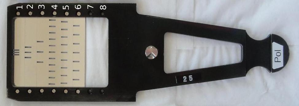
The choice of dekker position will depend on the nature of targets to be observed. The table below describes the characteristics of each dekker mask.
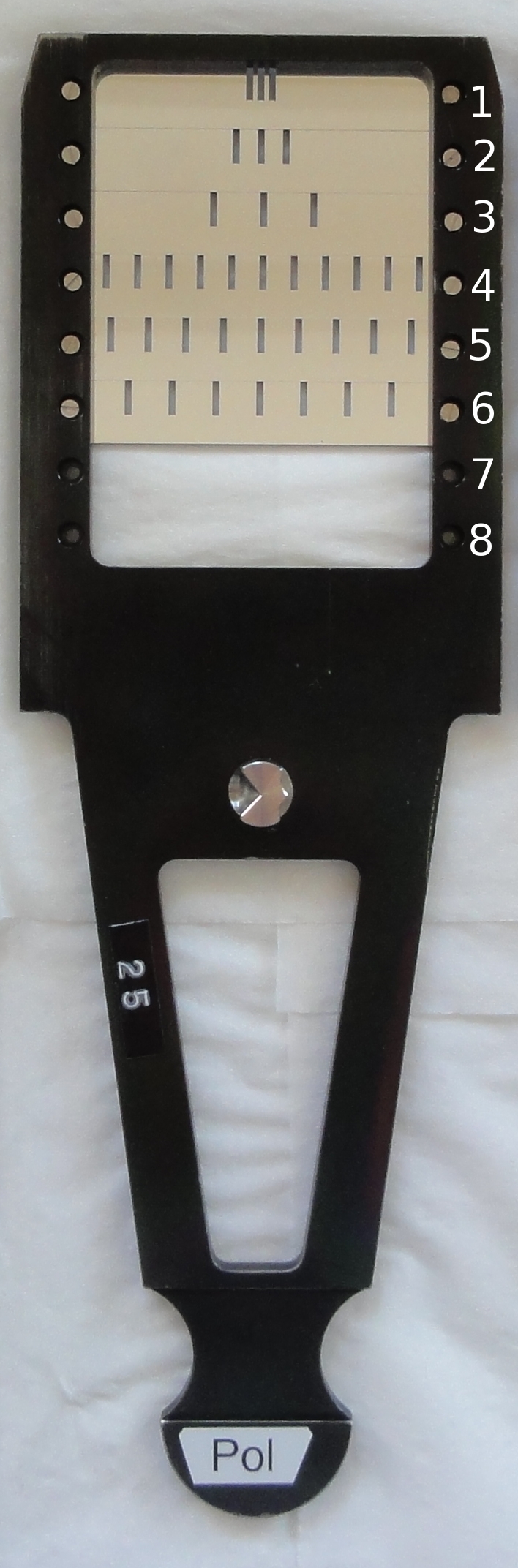
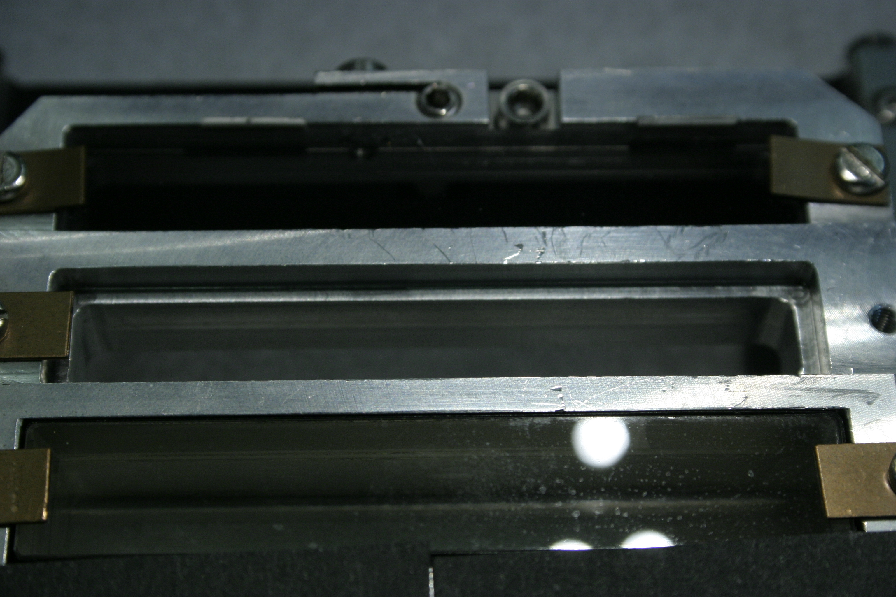
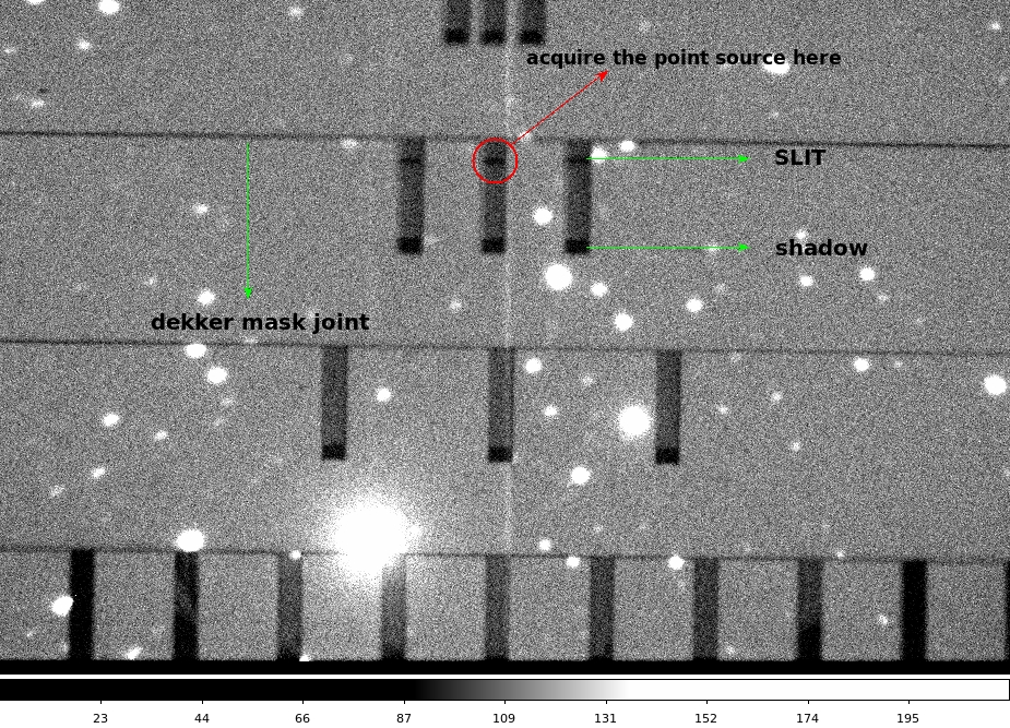
For point sources a dekker with three apertures, one for the source and two for the sky, can be used. Each aperture generates two beams. In the polarisation dekker slide, positions 1-3 have three apertures. The default option has the dekker slide in position 2 (ICS command "dekker 3"), in which the ordinary and extraordinary beams of the target and sky are aligned next to each other so that the CCD can be windowed to reduce the readout time. This default dekker-slide position has three apertures of 5 arcsec width, spaced by 18 arcsec. Therefore the total width is 41 arcsec, and the unilluminated space between the slots is 13 arcsec. The separation of the o and e rays is 8 arcsec. Dekker slide positions 1 and 3 are not usually used. Position 1 is a specially designed sky-compensation dekker (see page 23, section 5.3 of the Users' manual for more details). Position 3 was designed for FOS (The Faint Object Spectrograph), which is no longer in operation. Note that this dekker introduces additional vignetting when used with the quarter-wave plate. For extended sources the comb dekkers (in dekker slide positions 4-6) are used. They have different duty ratios, thus one has to plan in advance the size and number of position offsets along the slit to allow sampling of the full spatial extent of the slit. There are other comb dekkers on a different dekker slide, although these are rarely used. The analyserTo set the default position of the dekker (called POL18ARCSEC, which has a gap of 18 arcsec between the centre of the central dekker slot and the centre of the left or right dekker slot), type: SYS@taurus> dekker 3 Other dekker positions are listed here. Deploy the half-wave plate (for linear spectropolarimetry) or the quarter-wave plate (for circular spectropolarimetry) in the light path: SYS@taurus> hwin (for linear) or qwin (for circular) To take half-wave or quarter-wave plate out of the beam, type: SYS@taurus> hwout or qwout To move the Savart plate into the light path, type: SYS@taurus> fcp calcite To move the Savart plate out of the beam, type: SYS@taurus> fcp_out Set the appropriate window and readout speed of the detector in the usual way, using the windows below as a reference. But, these need to be checked empirically. SYS@taurus> window red 1 "[840:1190,1:4200]" SYS@taurus> window blue 1 "[890:1240,1:4200]" Take the usual set of calibrations described in the ISIS cookbook. For the flat fields use the same polarimetry components in the light path as for your observations, except for the dekker, for which it's recommended to take two sets of flat fields. The first set should be taken with the dekker slide in the clear position (type SYS@taurus> dekker 9). Next, insert your required dekker in the beam, and take another set of flat fields. Note that roughly double the exposure time will be needed compared to flat fields taken at dekker position clear; when the dekker slide is in the clear position each pixel is illuminated by both the ordinary and extraordinary rays. To take flat fields, set the half-wave (quarter-wave) plate to the angle where the contrast between the ordinary and extraordinary rays is minimized. For ISIS this is around 30.5 or 75.5 deg for linear, and around 185 deg for circular spectropolarimetry. If you want to take sky flat fields in addition to the tungsten lamp flat fields, ask the telescope operator to point the telescope to the Arago point (telescope azimuth = Sun azimuth - 180 deg and elevation ~ 20 deg at sunset), where the degree of the sky polarisation is close to zero. The Arago point lies about 20 deg above the antisolar point when the sun is close to (or just below) the horizon. It's important not to change any sensitivity parameters of the system between taking calibrations and science observations. This applies particularly to gratings, grating settings and filters. To find the focus of the telescope with ISIS for spectropolarimetric observations, follow the usual focusing procedure. Choose some bright star (a brighter star is needed than for the normal ISIS observations, e.g., V ~ 6-8 mag). The usual telescope focus is 0.2 (0.1) mm lower when using a half-wave (quarter-wave) plate compared to the ISIS focus without a wave plate. This means that the telescope focus will be around 97.65 and 97.75 mm for the linear and circular spectropolarimetry, respectively. Once the value of the focus is determined, set the value by, e.g., SYS@taurus> focus 97.65 If you are doing both linear and circular spectropolarimetry, it's recommended that you add all necessary focus changes to your observing scripts, or automate focus changes using a GUI hwp (qwp) "Dfocus" setting of -0.2 (-0.1) mm for linear (circular) spectropolarimetry observations. Make sure you determine the telescope focus well. An out-of-focus image can lead to polarisation effects if the image is sampled asymmetrically with the spectrograph slit. In this case, one samples a specific part of the primary mirror and will see a polarisation imprint due to the oblique incidence on that part of the mirror. With accurate focusing, all parts of the primary contribute equally, and the average polarisation effect is zero. It may be necessary to decrease the TV focus by 1500 microns and the autoguider focus by a few hundred microns. The telescope operator will take care of this. Point the telescope to your target and type: SYS@taurus> agslit Due to the thickness and field vignetting of the retarders they have to be retracted from the optical path to acquire a target: SYS@taurus> hwout (or qwout) After the acquisition is finished and auto-guiding is on, the wave plate can be inserted back into the beam: SYS@taurus> hwin (or qwin) In the acquisition camera you should see an image resembling the image below, where the vertical thick apertures are the dekker slots. Inside the dekker slots, and towards their lower extremes, it's possible to distinguish shadowed areas. These are the edges of the dekker, which are visible because of the 7.5 deg tilt of the dekker with respect to the slit-view camera (the slit jaws are inclined to the optical axis of the telescope at an angle of 7.5 degrees to allow the acquisition TV to view the reflected skylight off the polished slit jaws). At the upper extreme of the dekker slots there are thin horizontal lines visible. These are the interfaces of the metal plates of adjacent dekkers, visible in this image of the polarisation dekker slide. Finally, the dekker selected for observing has in the upper part of the slots
another shadowed area, which is the ISIS slit.
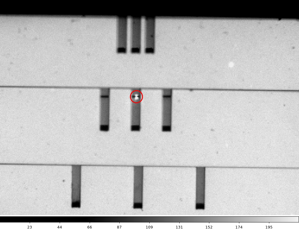
The target should be acquired in the intersection between the central dekker
slot and the ISIS slit, as shown
here.
Sometimes, particularly for bright targets, it's necessary to move the source out of
the ISIS slit to be able to see the dekker shape clearly.
Once the acquisition is complete, the telescope operator should close the autoguider loop (if necessary), and you can start your science exposures. Take data using the spectropolarimetry scripts located in /home/whtobs/isis_scripts: SYS@taurus> linpolscript <camera> <int time> <title> [nloop] (linear polarimetry) SYS@taurus> cirpolscript <camera> <int time> <title> [nloop] (circular polarimetry) where nloop is the number of loops, and defaults to one if not specified. Here are examples of scripts for linear and circular spectropolarimetry, which will take 4 and 2 images, respectively, at zero angles determined by your support astronomer. The zero angles are different for the red and the blue arm of ISIS, and also vary with other spectrograph settings like the central wavelength. Your support astronomer will modify the scripts to contain the correct zero angles for your run. Documentation for FIGARO is available
here,
documentation for TSP is available here, and documentation for convert is available
here.
figaro
In the example above the spectra are laid out in columns with the aperture A spectrum in columns 147 to 156 (ordinary) and columns 183 to 192 (extraordinary), and the aperture B spectrum in columns 228 to 237 (ordinary) and columns 264 to 273 (extraordinary). The two algorithms (OLD or RATIO) differ in the method used to compensate for transparency variations between the observations at two plate positions. The RATIO algorithm works very well on bright stars, but can fail on faint objects (or on 100% polarised calibration sources) through attempting to take the square root of a negative number. Under these circumstances the OLD algorithm should be used. The variances on the polarisation data are calculated from photon statistics plus readout noise. If you want to plot results, you can use the function PPLOT, which plots a polarisation spectrum: pplot Here is an example of the pplot input parameters:
Finally, if you want to calculate the polarisation P and the position angle Theta for a polarisation spectrum, use the PTHETA function: ptheta Here is an example of the ptheta input parameters:
The input in this example is in pixels. SYS@taurus> hwin (qwin), moves retarder plate in SYS@taurus> hwout (qwout), moves retarder plate out SYS@taurus> hwp <angle> (qwp <angle>), moves retarder plate to requested angle (0-360 deg) SYS@taurus> hwprot <rate> (qwprot <rate>), rotates retarder plate at requested rate (0 - 1 Hz) SYS@taurus> hwstop (qwstop), stops the rotation of retarder plate Continuous rotation for both half- and quarter-wave plates has a time-out of 12 hours (in case it's forgotten to stop it). Other useful commands SYS@taurus> fcp calcite, moves the Savart plate into beam SYS@taurus> fcp_out, moves the Savart plate out of beam SYS@taurus> dekker 3, chooses the standard position of the polarisation dekker SYS@taurus> mainfiltnd MF-POL-PAR, selects polariser in the main colour filter unit SYS@taurus> mainfiltnd 1, removes polariser in the main colour filter unit In case the retarder plates don't move, type: SYS@taurus> inhw (inqw), which initialises the half-wave (quarter-wave) plate. Reference system The angle of the half-wave and quarter-wave plate is relative to the instrumental reference. The orientation of the calcite block and the slit are fixed with respect to ISIS. So if the ISIS slit is at the parallactic angle, the angle of the retarder plate relative to north will depend on where on the sky the telescope points. A note on circular polarimetry Because the quarter-wave plate is not exactly quarter-wave for all wavelengths, the circular polarimeter is partly sensitive to linear polarisation. If you suspect linear polarisation in your source, you can depolarise it by continuous rotation of the half-wave plate ahead of the quarter-wave plate in the beam (which is default configuration of the retarders). This should eliminate systematic errors due to linear polarisation, and invert but otherwise leave intact, the true circular polarisation. If linear polarisation of your source is strong, you must determine to what extent the telescope converts linear to circular polarisation. The way to do this is to set up ISIS for circular polarisation, but observe a strongly linearly polarised star. Obtain two complete observations, with a rotator angle difference of 90 degrees. External circular polarisation will constant, but converted linear polarisation will be inverted in the two observations. Instrumental polarisation zero-point To 'depolarise' a zero-polarisation star completely, observe it twice, with a difference of about 90 degrees in rotator angle. In the Alt-Az frame, the average of the two observations represents the pure instrumental zero-point. The converse holds for a representation in the equatorial coordinate frame: the average is purely the stellar polarisation. Photon noise calculation An absolute error in the Stokes parameter ~ 1/√ N_total , where N_total is the number of photons per resolution element. So for example, in order to determine one Stokes parameter to a degree-of-polarisation accuracy of 0.005, 4x10⁴ photons per resolution element are required. To obtain both linear Stokes parameters with that accuracy, we need two such observations. For more details see Section 3.8.1 of the ISIS Spectropolarimetry Users' Manual. More information Some more information about ISIS spectropolarimetry can be found in the ISIS Spectropolarimetry Users' Manual. Although this is an old document and some specific detail isn't valid anymore, it contains invaluable background discussion on the broader aspects of spectropolarimetry with ISIS. |

| Top | Back |
|
