Fast Spectroscopy

1. Preliminaries
2. The L3CCD
3. The QUCAMs on ISIS
4. Observing with the QUCAMs

Two E2V electron multiplying ‘Low-Light-Level’ L3CCDs (i.e. the QUCAMS) are available for use on the red and blue arms of ISIS to do fast of faint-object spectroscopy. Both detectors are identical with 1k×1k, 13 microns/pixel, full frame transfer device, and can be used in two multiplying modes: slow or fast. In the fast mode the read-out-noise is nearly zero. Exposure times shorter than 1s are possible with almost no dead times (20 miliseconds per full transfer) as the system continuously expose while reading the previous image. The technical characteristics of QUCAM2 and QUCAM3 are summarized here (note that both detectors are nearly identical). The detectors have very good cosmetic characteristics, and excellent quantum efficiency.

The L3CCD differs from a standard CCD in the sense that it has a frame transfer buffer allowing quick transfer of accumulated charge (the image) into temporary on-chip storage, and it possesses and extended readout register where charge is amplified, allowing very high gains that make the classical read noise much less significant. Some important facts have to be taken into account to take advantage of their characteristics. A paper with more technical information and analysis of the noise sources can be found here. For some papers describing the use of L3CCDs please follow this link, and for sample images and observing tips for L3 cameras see this link.

2.1 Frame transfer CCD

With this frame transfer CCD it is possible to drastically reduce the time lost to reading out the chip. Charge is first rapidly shifted into a storage buffer in about 20 miliseconds. While the change resides in that buffer and is being read out, the exposure can just continue on the active CCD area. In this way observing efficiency is maximized.  During most recent tests (July 2007) exposure times of 0.229s using a 100 pixel-wide window over the full spectral length were achieved. Shorter exposure times are not possible as this is the time needed to read the buffer.

2.2 Electron multiplication and very low read noise

The electron multiplication takes place in an extra series of stages added to the serial register before the charge is digitized. These stages are clocked with higher than normal voltages, which leads to an avalanche of several hundred or even thousands of electrons for each electron that is collected on the chip. This then dwarfs the normal read out noise (RON) produced by the amplifiers. The resulting effective RON is close to zero (0.028 e- in the fast mode of our system).

The multiplication process introduces an adittional noise source called multiplication noise, see (Tulloch, 2007). In the detector noise limited regime (low signal levels) this loss is more than compensated by the negligible read noise of the system, but in the photon noise limited regime the multiplication noise reduce the SNR of the observation by a factor of 2^1/2 which is equivalent to say that the detector loses a factor of 2 in quantum efficiency.

2.3 Problems: linearity and CIC.

There are two special characteristics of L3CCDs that worth some attention.

Firstly, at high count levels non-linear behaviour occurs. The system is optimized to work with faint sources, so it is a good idea to keep the exposure time low to work always in a linear regime (<15.000 ADU/pixel).

Secondly, the high-gain amplification process generates occasional rogue electrons. This is the so-called "clock induced charges" (CIC). CIC is produced in all CCDs, but are only noticeable in an L3CCD due to the electron multiplying stage. The effect is that several "bight" pixels, randomly distributed, appear in the image (see Fig. 1). The number of CIC electrons is independent of the exposure time. 

Fig. 1: Zoom of an individual spectrum of 0.229s exp. time. Note the CIC events, which are shown as bright pixels randomly distributed all over the image.

2.3 Two observing modes.an>

The system has two modes with different multiplying factors at the extended readout register, fast and slow, with different gains (105 and 4.1 ADU/e) and RON (0.028 and 1.4e respectively). To take advantage of the almost 0 RON the best option is fast. But if the signal using the lowest possible exposure time using the fast mode is higher than 15000 ADU/pixels then the slow mode is recommended because of the non-linear behaviour high count levels and because the slow mode is less affected by CIC events.

3.1 Spectral resolution and wavelength coverage The spectrum is dispersed in the x axis. The L3CCD covers about 1/3 of the spectral range of that of the standard ISIS CCDs.

ISIS wavelength coverage and resolutions with QUCAM2/3 in the blue arm
Grating	Blaze	Dispersion (Å/mm)	Dispersion (Å/pix)	Total Spectral range (Å)	Unvignetted range (1024 pixels)	Slit-width for 54 mu at detector (in arcsecs)	Slit-width for 27 mu at detector (in arcsecs)
R158B	3600	120	1.56	1597	1597	0.8	0.4
R300B	4000	64	0.83	850	850	0.8	0.4
R600B	3900	33	0.43	440	440	0.9	0.45
R1200B	4000	17	0.22	225	225	1.1	0.55
H2400B	Holo	8	0.11	113	113	1.2	0.6

ISIS wavelength coverage and resolutions with QUCAM2/3 in the red arm
Grating	Blaze	Dispersion (Å/mm)	Dispersion (Å/pix)	Total Spectral range (Å)	Unvignetted range (1024pixels)	Slit-width for 54 mu at detector (in arcsecs)	Slit-width for 27 mu at detector (in arcsecs)
R158R	6500	121	1.57	1608	1608	0.84	0.42
R316R	6500	62	0.81	829	829	0.88	0.44
R600R	7000	33	0.42	430	430	0.97	0.48
R1200R	7200	17	0.26	266	266	1.24	0.62

Observing with the QUCAMs on ISIS is very similar to normal CCDs (see ISIS Cookbook). But some differences related only to the CCD operation are discussed below.

4.1 Settings.

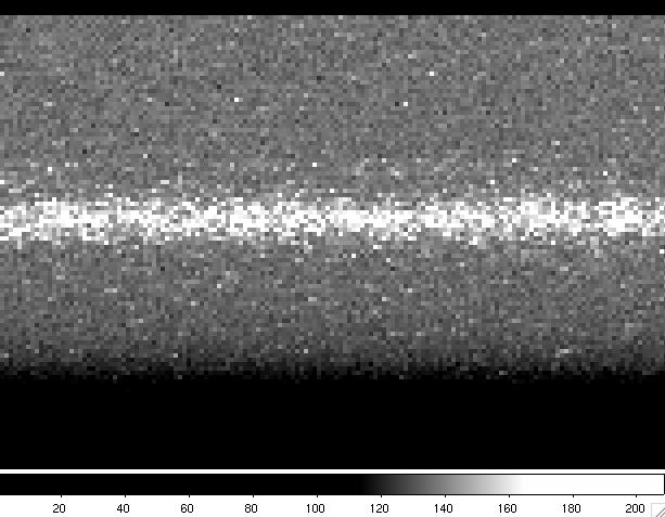
The spectral direction used with the QUCAMs is the x-axis. Windowing in the y-axis make read-out faster. To have enough sky at both sizes of a point-like source we used a window of 100 pixel width in y-axis and covering the whole range of the x-axis. In our tests we used

SYS> window 1 qucam2  "[1:1072,540:639] "

Windowing also in the x-axis permits shorter exposure times but the spectral range of the spectrum will be also shorter.


4.2 Taking spectra of the target.

All UltraDAS commands can be used as with the other CCD. But to continuously expose while reading the previous image the command to be used is rsrun.

rsrun performs a sequence of exposures for rapid spectroscopy on the camera, reads them out and saves the data in a FITS file containing the exposures in a sequence of FITS extensions. The file is passed to the archiving and logging facilities.

A title may be given for the observation: the title appears as the datum of the OBJECT keyword in the FITS headers and as the target name in the observing log. If no title is given, the system attempts to read the target name from the Telescope Control System (TCS): this makes the value for the OBJECT keyword the same as that for the CAT-NAME keyword. If the TCS does not respond, then the title defaults to "(object not named)".

rsrun [<camera>|<instrument>] <number-of-exposures> <exposure-time> ["<title>"]

multrsrun [<camera>|<instrument>] <n-obs> <number-of-exposures> <exposure-time>

where number-of-exposures is the required number of exposures in the sequence, exp-time is in seconds and n-obs is the number of cycles in a multrsrun. The title-string must be enclosed in double quotes.

Example:

rsrun red 127 1 "rapid spectroscopy run"

performs a series of 127 one second integrations.>

Note that the mechanical shutter is always open, thus if you use exp-time=0 the real exp. time depends on the time needed to make the full frame transfer (0.229s using a [1:1072,540:639] window)

A problem detected using rsrun is that the exposure-time of the individual images is not perfectly constant (see Fig. 3). As the camera is used with UltraDAS and this is not a real-time system, the full-frame transfer time depends on the other tasks the computer is running during the read-out process. This has to be taken into account when combining images to attain the final needed exposure time.



Fig. 3: Exposure time of the 200 individual images obtained using the rsrun command and 0 exposure-time. The plotted exposure time is measured as the difference between the utstart of two sucesive images. The red line corresponds to 0.229s, the minimum exposure time measured. Notice that the exposure time is not constant.

4.3 Bias, flats, arcs.

Arcs and bias can be obtained in the usual way. Flat fields have to be obtained at low-signal levels (less than 10000 ADUs), so to attaing good S/N several flat fields are needed.