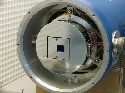
Observers should be aware of important differences between these cameras and other conventional cameras that they may have used at ING.

New Command Syntax
In addition to all the usual uDAS commands , we have introduced some new ones to allow better performance in the application of rapid spectroscopy. Previously uDAS has suffered from very bad timing jitter when taking sequences of rapid spectra. We have now offloaded the timing task from the SPARC  into the SDSU controller where the timing is now locked to a crystal oscillator. These new commands supersede the earlier 'rsrun' command.

The new commands (currently available only on the QUCAMs) are as follow:

    rmode spec <n_reads>
    rmode simple
    run, glance, scratch etc.

To enable the rapid spectroscopy readout mode for the camera, the command 'rmode spec <n_reads>' is used. For example to set the camera up to perform 360 readouts:

rmode qucam2 spec 360

Once the readout mode is set, the normal run commands (run, glance, scratch etc.) are used to perform exposures. The time specified in the run command is then used as the integration time for each readout in the readout sequence e.g.

run qucam2 5 - perform a sequence of 5 second exposures, with the number of exposures determined by the n_reads parameter used in the 'rmode spec <n_reads>' command.

The time taken to perform a rapid spectroscopy run will be approximately:

t = n_reads * (exposure_time + readout_time)

To disable the rapid spectroscopy readout mode for the camera, set the readout mode back to simple:

rmode qucam2 simple

Image sequences obtained using 'rmode spec' are stored in a single fits file with extensions.

NOTE:  zero second exposures are not permitted. 1ms is the minimum requested exposure time.

Calculating Exposure Times
Exposures for the L3 cameras are timed using the processor clock of the SDSU controller. the crystal clock is specced to 100ppm across its whole temperature range. Since the temperature of the controller is pretty stable, the actual timing accuracy will be a lot better than this.
 When doing  'rmode simple' exposures there will be a timing error (probably at the level of 10s of ms)  associated with the opening and closing of the mechanical shutter and this will dominate. When doing image sequences using the 'rmode spec' command timing will be much better.

There is an important feature of frame transfer operation that the observer should be aware of. When using the 'rmode spec' command to do a sequence of spectra. If for example we request the following:


Latency between image sequences
As each image sequence run progresses, the pixel data is stored in a raw format in a buffer. At the end of the run this data is then assembled into a multi-extension fits file and written to the obsdata disc. This takes 50s for a 388MB image sequence. During the first 16s of this period the DAS is processing the image and a new run cannot be started. After 16s the observer can commence a new run.

Data Volume
If image sequences with minimum exposure time of 1ms are taken, the data rate will be 592KByte per second or approximately 1GByte per 30 minute observation. Runs of greater than 30 minutes or with data volumes greater than 500MB are not recommended.

Time Stamps
A time stamp is obtained from the ING timeserver at the start and end of each 'rmode spec'  sequence. A timestamp is then calculated by interpolation for each of the frames in the sequence and inserted into each frame's header in the 'UTSTART' field. The absolute accuracy of this timestamp is 1ms.
A link to the ING timeserver webpage can be found here
An example header can be found here

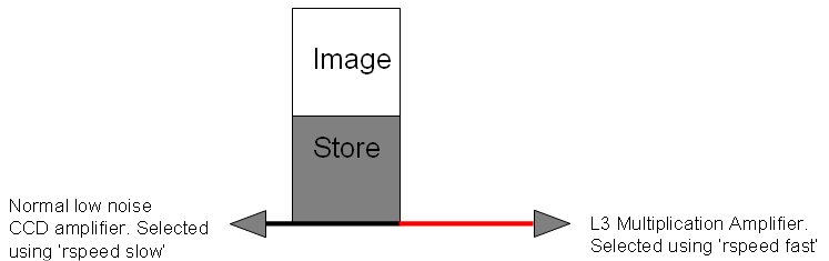
Amplifier Selection
The L3 CCDs have 2 amplifiers. One is a conventional low noise amplifier with very similar characteristics to the EEV and RED+ cameras. This conventional amplifier can be selected by using the 'rspeed slow' command prior to doing a run. This amplifier is preferred if the observations are to be photon noise rather than detector noise limited. The second amplifier uses avalanche multiplication in an 'L3 register' to give read noise of <<1e. It can be selected by using the 'rspeed fast' command prior to doing a run. It is preferred for observations that would otherwise be detector noise limited. The noise of this amplifier is sufficiently low to easily allow the detection of single photons and as  the object brightness falls , the image can be seen to break up into discrete spots, each corresponding to a single photo-electron.


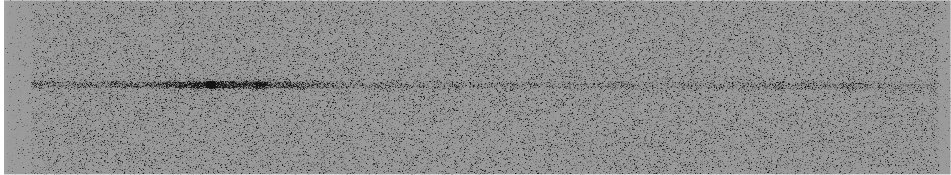
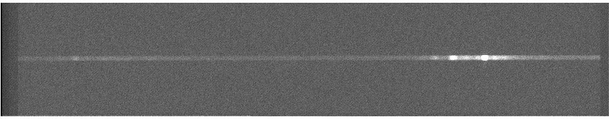
Since the readout amplifiers are positioned on opposite sides of the CCD, when switching between amplifiers the observer will notice that the images become mirrored. This effect is shown in the two spectra below. These were obtained on ISIS Blue arm with QUCAM2


5 second exposure. L3 amplifier selected


60 second exposure. Normal amplifier selected

Frame Transfer Operation
In addition to having L3 architecture, the QUCAMs also have a frame transfer geometry. If the observer is  doing 'rmode simple' exposures then they will notice no difference compared to a normal CCD readout ; the exposure will be mechanically shuttered just like a normal science camera. For image sequences taken with the 'rmode spec' command, however, the FT operation is fully utilised. The mechanical shutter is only operated at the very start and end of the sequence. The exposure time of the individual frames is then defined by the frame transfer operation where the image are is rapidly shifted under a light tight store area from where it is more leisurely read out whilst the next frame is exposing. The CCD is therefore exposing almost continuously  and makes maximum use of the light delivered by the telescope. With very bright sources and  very short exposure times , vertical streaks above and below the  highlights may become visible in the image. These are artifacts of the frame transfer process. Frame transfer takes 15ms.

Windowing
Windowing in X is not recommended since it will reduce the gain of the system. Windowing in Y has no such effect. This is unlikely to be a limitation since in the case of QUCAM2 the spectral axis is horizontal and already has a fairly limited extent due to the small CCD size. Windowing in Y will be useful for reducing data volume and increasing readout speed. It will have no effect on the noise,CIC or gain.

Binning
Only Y binning has been implemented . On-chip binning is not generally recommended for L3 observations except to reduce read out  times. In a conventional CCD , binning offers a noiseless method of adding pixels. Since the read noise of an L3 chip is close to zero , any binning can be accomplished post-readout with very little penalty. Post-readout binning can then be done in a flexible manner.

Aborting
An abort in mid run will take no longer than the frame cycle time + 12s  to return the observing system prompt.

Clock Induced Charge
Some stray charge is generated inside the CCD by the clock transitions. All CCDs display this but it is generally swamped by the read noise. In L3 CCDs the CIC is clearly visible as a random sprinkling of single photo-electron events. The effect is very like that of a faint background. CIC is independent of exposure time. QUCAM2 has a CIC of about 0.035 electrons per pixel, meaning that about 1 in 30 pixels will contain an electron of CIC.

Multiplication Noise
This is an additional noise source introduced by the L3 multiplication process. It acts to amplify the Poissonian photon noise by a factor of root(2). In the photon noise limited regime this can be equated with an effective 50% loss in quantum efficiency. Multiplication noise means that a single electron entering the multiplication register can give a whole range of possible output values. The graph below shows a histogram of pixel values found in a very weakly iluminated flat field (the mean illumination being <<1 photon per pixel).


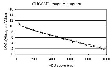
What the graph shows is that a single electron can generate a signal of anywhere between 1 and >1000 ADU of output. Incidentally, the gradient of the linear portion of this histogram can be used to calculate the gain of the system. The gradient = -1 x system gain in units of input electrons per output ADU. Note the log base e vertical scale.


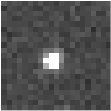
Charge Transfer Efficiency
Cosmic rays typically leave a large horizontal trail in the image indicative of poor horizontal charge transfer efficiency. This is due to the charge carrying capacity of the L3 register being exceeded during the multiplication process. At lower signal levels, for which these cameras are optimised, poor CTE is not a problem. This was tested using a laboratory pinhole focussed into a spot with a FWHM of <2pixels. The peak amplitude of the spot was approximately 300 electrons i.e. approaching the top of the dynamic range of the camera when in L3 mode. The spot image was examined for elongation when read out through both the conventional and L3 amplifiers. The image was then analysed using a 2D Gaussian fitting program to measure the FWHM in both axes.

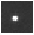Normal Amplifier	L3 Amplifier

As can be seen by eye the images do not display any horizontal trailing. The Gaussian fitting program gave the following results:

   
Gain Stability
The conventional amplifier should have a very stable gain close to 0.97e/adu. There will only be a very weak temperature dependence and ageing effect. The L3 amplifier on the other hand has a very high temperature coefficient of about -4% per degree K. When the camera is still in the process of cooling down the gain will be considerably lower than that stated on the web page. Gain calibration frames should be taken at intervals throughout an observing run. These can be stacks of bias frames that can be later analysed using the histogram method described above. Alternatively if the science frames contain generous un-illuminated areas, these will contain enough CIC events to allow each individual frame to be used for gain calibration. An alternative method for monitoring L3 gain changes is to observe a stable source (for example a calibration lamp) through the conventional amplifier before swapping back to the L3 amplifier. The conventional amplifier is known to be very stable and can be used to calculate accurately the source brightness. The gain stability has been tested in the laboratory using a stable pinhole source. It's image was defocussed so as to allow a brighter source to be used without saturating the CCD. The graph below shows the integrated brightness of the pinhole image during two consecutive 30minute 'rmode spec' runs. Each run consisted of 360 5second exposures. It demonstrates gain stability as well as the absence of timing glitches in the cadence of the exposures.



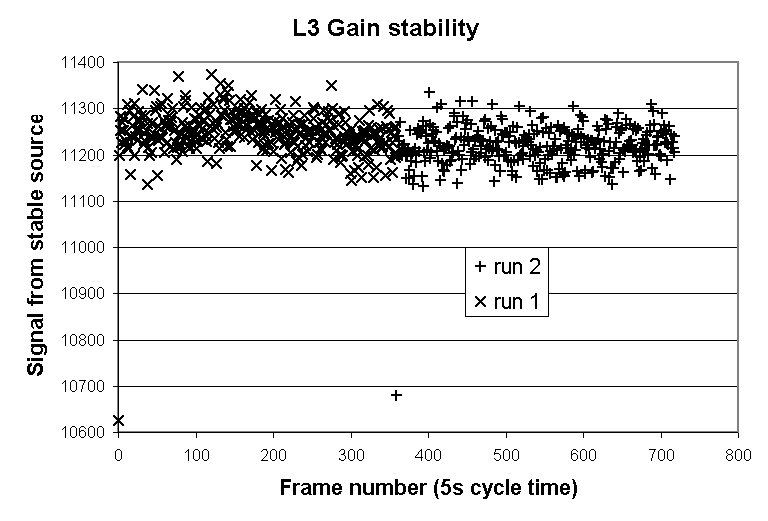
The first frame in each run appeared to have an exposure of about 6% less than the rest of the run. The observed brightness of the source (discounting these initial frames) during the full 1 hour observation had a standard deviation of  0.5%

Photon Counting
If the images are not too deeply exposed (<0.1 photo-electrons per pixel on average) then it is possible to do photon counting. A threshold is applied to the images and any pixels over that limit are interpreted as containing 1 photon. This has the benefit of removing multiplication noise. Some care must be exercised in the choice of threshold. If too high then the effective QE will suffer as some photo-electron events will fall under the bar. If set too low, then read noise will cause false triggers. The read noise is about 3-4ADU , the average height of a photo-electron is about 116 ADU. Setting the threshold to about 20 ADU (above bias mean) would be  a good starting point. In the case of a spectra containing both strong and faint emission lines it should even be possible to apply photon counting analysis to the faint line and proportional analysis to the stronger.

Pros and cons of using the L3 amplifier
The ability to do temporal, spectral and spatial binning post-readout is a great advantage in an L3 CCD. These can all be accomplished with minimal noise penalty. Generally speaking any application that would otherwise be readnoise limited is best done with an L3 detector. One obvious application would be the detection of very faint emission lines.  If the application is photon noise limited then it will generally be better to use a conventional detector since it does not suffer from multiplication noise. The nice thing about the QUCAMs is that they have the flexibility to be used in both conventional and L3 mode depending on which speed is selected..

Links

Quick Look Data Reduction Software for QUCAM2

Monte Carlo Modeling of L3 detectors in High Time Resolution Applications, HTRA Edinburgh Sep 2007 (pdf)

Photon Counting and Fast Photometry with L3 CCDs. SPIE5492-173 Glasgow 2004, Simon Tulloch (pdf)

Photon Counting Stategies with L3 CCDs , A.Basden

Sub Electron noise at MHz pixel rates, Craig Mackay, SPIE 43061 (pdf)

Powerpoint presentation on L3 detectors (includes section on Deep Depletion CCDs also)

---

Simon Tulloch Jan 2008