1. Introduction
2. Rapid spectroscopy mode (RSM)
3. Defining the setup
4. RS mode in practise
5. Timing and overheads
6. Problems and limitations
Very small dead times on CCD exposures are in some cases essential to achieve the scientific objective of observing programmes, particularly for high-speed time-resolved observations. For instance in the study of close binary stars or flare stars, long time series with exposure times of the order of a second are required. The period between exposures has to be kept as short and regular as possible in order for the experiment to be efficient, or even feasible.
A standard CCD exposure on the WHT data acquisition system introduces approximately 9 seconds of dead time for chip clearing, shutter control, file creation, system communication etcetera. This time loss is in addition to the time it takes to read out the CCD. Such a delay renders high-speed time-resolved work very inefficient. For exposure times of the order of a second or less an additional problem is encountered in the fact that the mechanical shutter is relatively slow to respond. This results in a variable exposure across the field. Apart from this, large numbers of short exposures, as is usually required in high-speed observations, would cause severe mechanical wear to the shutter.
The standard data acquisition system (uDAS) on the William Herschel Telescope on La Palma has been upgraded to include the Rapid Spectroscopy mode, which is specifically designed to allow very fast continuous readout of a windowed area of the CCD with minimal dead time. The shutter remains open during this process. Between individual frames the CCD is only partly cleared to further reduce dead time. This partial clear involves a rapid shift of the image by 35 rows ; slightly larger than the height (in the spatial direction) of the spectrum on the CCD. This new mode replaces the 'Drift Scan Mode' (see Jorden and Maclean, 1994, RGO internal technical note, and the old user Manual), previously offered with the old Dutch DAS.
The description below gives a more detailed account of the practical aspects of using the Rapid Spectroscopy Mode. This mode is ONLY available for TEK4, but could be extended to other TEK chips. It cannot be applied to any EEV device.
2. Rapid spectroscopy mode (RSM)
Since in the Rapid Spectroscopy Mode the shutter does not close while the windowed region of the CCD is read out, some smearing of the image will occur. The readout process involves a rapid shift of the windowed area (that contains the spectrum) into a non-illuminated part of the CCD from where it can be read out in a more leisurely fashion. This illuminated area of the CCD is defined by an above-slit Dekker. The light falling on the CCD is restricted to an area extending the full width (the spectral direction) of the chip but with a vertical (spatial) extent of only 35 rows. It is during this rapid shift that some vertical smearing will occur. Prior to an exposure, the partial clear will also introduce some additional smearing. The overall effect is that each line in the image will have been exposed to signal from all the other lines for a total of about 5 ms. This will not be a problem except for exposures that last only a few hundred milliseconds.
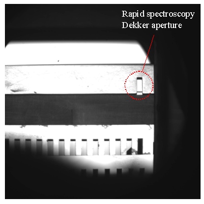
The first step in using the rapid spectroscopy mode is to define the area-of-interest on the CCD. The area outside this region has to be masked off. In the case of ISIS the masking is best done with a dekker aperture. An slot of 12 arcsec in length is available in dekker A position 7. Figure shows an image of the dekker taken with the TV camera (TVSCALE 12, display zoomed out 2:1, dome lights on). The Dekker aperture is only visible on the aquisition camera when TVSCALE 12 is selected.
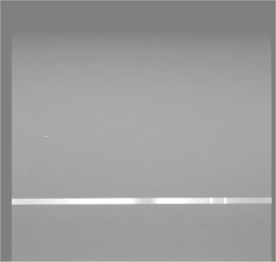
window red 1 "[1:1100,225:260]" should be ok for the red arm of ISIS and dekker A in position 7. Sometimes, positioning errors when the camera is remounted can change the window. In any case, we recommend the observer does a normal full frame run to stablish the optimum window position. Next figure shows a full TEK4 frame image (dome light spectrum) taken with the ISIS RED arm and the dekker A slide in position 7.
There's no special command to switch to rapid spectroscopy mode. The rsrun command allow a get rapid spectroscopy. At least the UltraDAS S9-4 version of the CIOS should be running. This mode is ONLY available for TEK4, but could be extended to other TEK chips. It cannot be applied to any EEV device.
Next, one has to define the window (see previous section) of interest on the CCD, binning, and readout speed through the WINDOW, BIN, and RSPEED commands. Slow and fast readout speeds can be used, and the characteristics are identical to operation in normal mode.
The number of exposures must be less than 128 in the RS mode.
Then to start a sequence of exposures type:
RSRUN [<camera>|instrument] <number_of_exposures> <exposure-time> ["<title>"]
e.g.: RSRUN RED 127 1
This command performs 127 x 1 second integrations
Valid integration times are between 0.2 and 15 seconds. The number of integrations must not exceed 128.
Once the integration has started, the data is read out one exposure at a time. For each exposure the time is reported on the chip box information. At the end of the run, the data is saved onto the disk, in a FITS file with <number_of_exposures> extensions, each containing all the usual header items. Further exposures with the same setup can just be started with the RUN command.
To interrupt a RS run one may use the abort command. The sequence of exposures will stop. The effect of the finish command during a RS run is still undefined.
With RS run experiments it is common to require (relative) photometric calibration of the data on short time scales. This can be accomplished by monitoring a second star on the same science frame. However, when a second star can not be accommodated two options are available to achieve correction for variable slit losses and sky transparency variations. When the slit width is matched to (or smaller than) the seeing, variations in the recorded counts will be dominated by seeing variations. A way to correct for this would be to correlate the FWHM of the star image with the total flux in each spectrum. This will give a curve which relates seeing to slit losses, which can subsequently be used to correct each exposure for slit losses. Alternatively, one could use the automatically logged autoguider data to later correct for sky transparency variations. The success of these corrections will depend on a combination of (sometimes time variable) factors such as seeing, sky transparency, telescope tracking and guide errors, and slit width. It is advisable to conduct some experiments to find the most suitable solution.
The autoguider relative transparency (and the seeing) is measured approximately every 10 seconds, and the information is stored on DISK$WHTDATA2:[SEEING] in an ASCII file Ayymmdd.WHT . One may ftp that data for later use.
Timing of the RS exposures is done by the DAS computer, while the sequencing
of the exposures is performed by the ICS computer. Each individual fits
extension contains header items which accurately record the actual time
and duration of the exposure. The information shown below were measured
using a rsrun on a TEK 1k x 1k CCD (TEK4) with a window of 1100 x 50 pixels
at the botton region ([1:1100,205:255]) of the chip. The number of
exposures were 60 and the demand integration was 1 second. The actual integration
time averaged 1.02s with an rms of 4.42ms, and the cycle time for each
exposure averaged 1.67s with a rms of 5ms.
| Integration time demanded | 1s | Readout cycle time: | |
| Mean | 1.021300533 | Mean | 1.670118644 |
| Standard Error | 0.0001113 | Standard Error | 0.000125816 |
| Median | 1.021298 | Median | 1.67 |
| Standard Deviation | 0.000862129 | Standard Deviation | 0.000966414 |
| Sample Variance | 7.43267E-07 | Sample Variance | 9.33957E-07 |
| Kurtosis | 1.171371792 | Kurtosis | 1.304640696 |
| Skewness | 0.014470997 | Skewness | 0.111136583 |
| Range | 0.00442 | Range | 0.005 |
| Minimum | 1.019183 | Minimum | 1.668 |
| Maximum | 1.023603 | Maximum | 1.673 |
| Sum | 61.278032 | Sum | 98.537 |
We would appreciate any feedback Observers have on fast spectroscopy
mode with ISIS.