1. Preliminaries
2. The L3CCD
   
3. QCAM2 at ISIS
   
4. Observing with QCAM2 on ISIS
   

Back to the top

2.1 Frame transfer CCD

With this frame transfer CCD it is possible to drastically reduce the time lost to reading out the chip. Charge is first rapidly shifted into a storage buffer. While the change resides in that buffer and is being read out, the exposure can just continue on the active CCD area. In this way observing efficiency is maximized.  During most recent tests (July 2007) exposure times of 0.229s using a 100 pixel-wide window over the full spectral length were achieved.  Shorter exposure times are not possible as this is the time needed to read the buffer.

2.2 Electron multiplication and very low read noise

The electron multiplication takes place in an extra series of stages added to the serial register before the charge is digitized. These stages are clocked with higher than normal voltages, which leads to an avalanche of several hundred or even thousands of electrons for each electron that is collected on the chip. This then dwarfs the normal read out noise (RON) produced by the amplifiers. The resulting effective RON is close to zero (0.028 e- in the fast mode of our system).

The multiplication process introduces an adittional noise source called multiplication noise (see  Tulloc 2007). In the detector noise limited regime (low signal levels) this loss is more than compensated by the negligible read noise of the system, but in the photon noise limited regime the multiplication noise reduce the SNR of the observation by a factor of 2^1/2 which is equivalent to say that the detector loses a factor of 2 in quantum efficiency.

2.3 Problems: linearity and CIC.

There are two special characteristics of L3CCDs that merit some attention.

Firstly, at high count levels non-linear behaviour occurs. The system is optimized to work with faint sources, so it is a good idea to keep the exposure time as low to work always in a linear regime (<15.000 ADU/pixel).

Secondly, the high-gain amplification process generates occasional rogue electrons. This is the so-called "clock induced charges" (CIC). CIC is produced in all CCDs, but are only noticeable in an L3CCD due to the electron multiplying stage. The effect is that several "bight" pixels, randomly distributed, appear in the image (see Fig. 1). The number of CIC electrons is independent of the exposure time.  The best way to deal with is to median filter a number of identical images. Since the RON is very low this does not negatively impact on the signal-to-noise of the end result. The exposure time can be kept low in order to obtain a reasonable number of exposures within the required time resolution dictated by the scientific goals. An example of the end result is shown in Fig. 2.

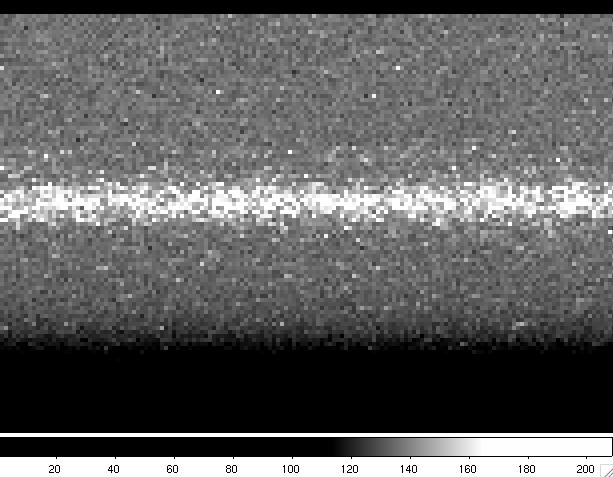
Fig. 1: Zoom of an individual spectrum of 0.229s exp. time. Notice the CIC events as bright pixels randomly distributed all over the image

Fig. 2: Zoom of a median combination of 11 spectra, each of 0.229s exp. time.  Notice that the CIC events have disappeared.

2.3 Two observing modes.

The system has two modes with different multiplying factors at the extended readout register,  fast and slow, with different gains (105 and 4.1 ADU/e) and RON (0.028 and 1.4e respectively).  To take advantage of the almost 0 RON the best option is fast. But  if the signal using the lowest possible exposure time using the fast mode is higher than 15000 ADU/pixels then the slow  mode is recommended because of the non-linear behaviour high count levels and because the slow  mode is less affected by CIC events.

Back to the top

3.1 Spectral resolutions and wavelength coverage

The spectrum is dispersed in the x axis. The L3CCD covers about 1/3 of the spectral range of that of the standard ISIS CCDs.

Observing with the QUCAM2 on ISIS is very similar to that the normal CCDs (see ISIS Coockbook). But some differences related only to the CCD operation are discussed below.

4.1 Settings.

The spectral direction used with QUCAM2 is in the x-axis. Windowing in the y-axis make read-out faster. To have enough sky at both sizes of a point-like source we used a window of 100 pixel width in y-axis and covering the whole range of the x-axis. In our tests we used

SYS> window 1 qucam2  "[1:1072,540:639] "

Windowing also in the x-axis permits shorter exposure times but the spectral range of the spectrum will be also shorter.


4.2 Taking spectra of the target.

All UltraDAS commands can be used as with the other CCD. But to continuously expose while reading the previous image the command to be used is rsrun.

rsrun performs a sequence of exposures for rapid spectroscopy on the camera, reads them out and saves the data in a FITS file containing the exposures in a sequence of FITS extensions. The file is passed to the archiving and logging facilities. 

A title may be given for the observation: the title appears as the datum of the OBJECT keyword in the FITS headers and as the target name in the observing log. If no title is given, the system attempts to read the target name from the Telescope Control System (TCS): this makes the value for the OBJECT keyword the same as that for the CAT-NAME keyword. If the TCS does not respond, then the title defaults to "(object not named)".

   rsrun [<camera>|<instrument>] <number-of-exposures> <exposure-time> ["<title>"]

   multrsrun [<camera>|<instrument>] <n-obs> <number-of-exposures> <exposure-time>

where number-of-exposures is the required number of exposures in the sequence, exp-time is in seconds and n-obs is the number of cycles in a multrsrun. The title-string must be enclosed in double quotes.

Example:

    rsrun red 127 1 "rapid spectroscopy run"

performs a series of 127 one second integrations.

Notice that the mechanical shutter is always open, thus if you use exp-time=0 the real exp. time depends on the time needed to make the full frame transfer (0.229s using a [1:1072,540:639] window)

A problem detected using rsrun is that the exposure-time of the individual images is not perfectly constant (see Fig. 3). As the camera is used with UltraDAS and this is not a real-time system, the full-frame transfer time depends on the other tasks the computer is running during the read-out process. This has to be taken into account when combining images to attain the final needed exposure time.









Fig. 3: Exposure time of the 200 individual images obtained using the rsrun command and 0 exposure-time. The plotted exposure time is measured as the difference between the utstart of two sucesive images. The red line corresponds to 0.229s, the minimum exposure time measured. Notice that the exposure time is not constant.

4.3  Bias, flats, arcs.

Arcs and bias can be obtained in the usual way. Flat fields have to be obtained at low-signal levels (less than 10000ADUs), so to attaing good S/N several flat fields are needed.

Back to the top

---

Last Updated: September 2007 Javier Licandro, licandro@ing.iac.es