1. Preliminaries
2. The L3CCD
   
3. QCAM2 at ISIS
   
4. Observing with QCAM2 on ISIS
   

Back to the top

2.1 Full frame transfer CCD

2.2 Electon multiplying system with almost 0 ron.


This is also an electron multiplying system.  They have an extra series of stages added to the serial register before the charge reaches the amplifier. This stages are clocked with higher than normal voltages which creates a significant probability that one electron will generate another as the charges are moved from stage to stage so a single electron lead to an avalanche of several hundred or even thousands of electrons. This dwarf the read out noise (ron) produced by the amplifiers, thus the ron is almost 0 (0.028 e- in the fast mode of our system).

2.3 Problems: linearity and CICs.


The system has two problems. First is the non-linearity  at high count levels. The system is designed to work wit faint sources, so it is a good idea to keep the exposure time as low as possible to work always in a similar regime.

The other problem are the so called "clock induced charges" (CICs). These are spontaneously produced electrons during clocking. CICs are produced in all CCDs, but are only a problem in an L3CCD due to the electron multiplyin stage. The effect is that several "bight" pixels randomly distributed, appear in the image (see Fig. 1). The number of CICs is independent of the exposure time, each image will have a similar number of CICs but at different pixel positions.   So, the best way to deal with is, again, to keep the individual exposure time as lower as possible, anf as the ron is almost 0, then combine the large number of images possible to attain the needed time resolution as in Fig. 2.

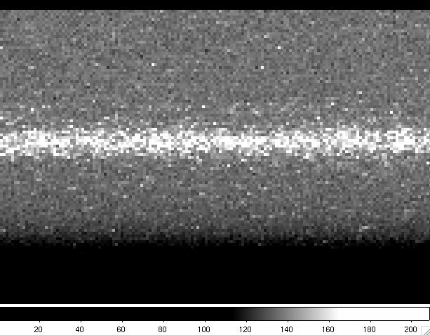
Fig. 1: Zoom of an individual spectrum of 0.229s exp. time. Notice the CICs ("bright" pixels randomly distributed all around the image).

Fig. 2: Zoom of 10 spectra, each of 0.229s exp. time.  Notice that CICs

2.3 Two observing modes.


The system has two modes with different multiplying factors, fast and slow. To take advantage of the almost 0 ron the best option is "fast". The "slow" mode is less affected by CICs, but it is only recommended if the signal using the lowest possible exposure time is higher than 20e/pixel.
"Fast" mode can be used also as a "photon counting" detector if the signal is slower than 0.2e/pixel. We still did not test this.

Back to the top

3.1 Spectral resolutions and wavelength coverage

The spectrum is dispersed in the x axis. Even if the L3CCD is about 1/4 size respect to the "normal" CCDs used on ISIS, the spectrum is not vignetted so the spectral coverage is about 1/3 of that of the normal CCDs.

Observing with the QUCAM2 on ISIS is alsmost as with the normal CCDs (see ISIS Coockbook). But some differences related only with the CCD operation are discussed below.


4.1  Settings.

The spectral direction used with QUCAM2 is in the x-axis. Windowing in the y-axis make read-out faster. To have enough sky at both sizes of a point-like source we used a window of 100 pixel width in y-axis and covering the whole range of the x-axis. In our tests we used

SYS> window 1 qucam2  "[1:1072,540:639] "

Windowing also in the x-axis pemit shorter exposure times but the spectral range of the spectrum will be much shorter.



4.2  Takking spectra of the target.

All UltraDAS commands can be used as with the other CCD. But to continuously expose while reading the previous images the command to be used is rsrun.


rsrun performs a sequence of exposures for rapid spectroscopy on the camera, reads them out and saves the data in a FITS file containing the exposures in a sequence of FITS extensions. The file is passed to the archiving and logging facilities. 

A title may be given for the observation: the title appears as the datum of the OBJECT keyword in the FITS headers and as the target name in the observing log. If no title is given, the system attempts to read the target name from the TCS: this makes the value for the OBJECT keyword the same as that for the CAT-NAME keyword. If the TCS does not answer, then the title defaults to "(object not named)".

   rsrun [<camera>|<instrument>] <number-of-exposures> <exposure-time> ["<title>"]

   multrsrun [<camera>|<instrument>] <n-obs> <number-of-exposures> <exposure-time>

where number-of-exposures is the required number of exposures in the sequence, exp-time is in seconds and n-obs is the number of cycles in a multrsrun. The title-string must be enclosed in double quotes.

Example:

    rsrun red 127 1 "rapid spectroscopy run"

performs a series of 127 one second integrations.

Notice that the mechanical shutter is always open, thus if you use exp-time=0 the real exp. time depends on the time needed to make the full frame transfer (0.229s using a [1:1072,540:639] window)

A problem detected using rsrun is that the exposure-time of the individual images is not constant (see Fig. 3). As the camera is used with UltraDAS and this is not an stand-alone system, the full-frame transfer time depends on the other tasks the computer is runing during the read-out process. This has to be takken into account when combining images to attain the final needed exposure time.






Fig. 3: Exposure time of individual images obtained using the rsrun command and 0 exposure-time. The plotted exposure time is measured as the difference between the utstart of two sucesive images. The red line corresponds to 0.229s, the minimum exposure time measured. Notice that the exposure time is not constant.

4.3  Bias, flats, arcs.

 
Arcs and bias can be obtained in the usual way. Flat fields have to be obtained at low-signal levels (less than 2000ADUs in fast), so to attaing good S/N several flat fields are needed.

Back to the top

---

Last Updated: Agust 2007 Javier Licandro, licandro@ing.iac.es