Photometric Redshifts: A Comparison of Methods - ING Newsletter No. 3, September 2000

THE ING NEWSLETTER No. 3, September 2000

GENERAL SCIENCE TELESCOPES AND INSTRUMENTATION OTHER NEWS FROM ING TELESCOPE TIME

Previous: Lithium Trail Leads Back to the Big Bang Up: Table of Contents Next: First Light of INGRID on the WHT !

Other available formats: PDF | gzipped Postscript
Photometric Redshifts: A Comparison of Methods
^{Dan Batcheldor*
(ING and University of Hertfordshire) and Nic Walton (ING)}
^{*: Daniel Batcheldor
is currently undertaking a placement year at the ING from the University
of Hertfordshire. He is studying for an Honors degree in Astronomy and
is due to graduate at the end of 2001.}
The advantages of being able to accurately extract red-shifts from photometric data is of great importance when wanting to complete large scale surveys of the night sky. In an exposure of minutes, rather than the hours needed for spectroscopy, we are able to gain colour data from a great number of astronomical sources at once. This is especially apparent with the advent of large format panoramic cameras such as the INT WFC, MegaCam at the Canada-France-Hawaii Telescope (CFHT) and, in the future, VISTA (Visible & Infrared Survey Telescope for Astronomy). If this data can then be used to accurately calculate the distribution of galaxies with red-shift, the large scale structure of the universe can be more readily determined.
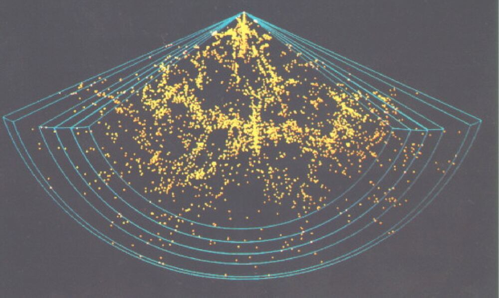
Views of large scale structure have revolved around the 'Swiss cheese' analogy. Geller and Huchra (1989) showed that clusters of galaxies themselves tend to form in bubbled patterns enclosing empty regions measuring hundreds of millions of parsecs across (see Figure 1). The Swiss cheese model has also been explored by Moore et al. (1992), but consists of a 'meat-ball' distribution in a void background (see Figure 2).

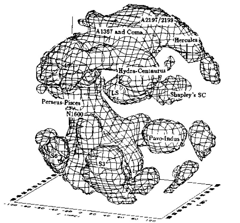Figure 1. Distribution of ~4000 galaxies in red-shift space, Geller and Huchra (1989). [ JPEG | TIFF ] Figure 2. Distribution of galaxies within 100Mpc of the Milky Way, Moore et al. (1992). [ JPEG | TIFF ]

There are two techniques that can be used when wanting to carry out red-shift calculations from photometric data; template fitting and the use of a training set. The first technique was initiated by Baum (1962) and later developed by Koo (1985) and Loh & Spillar (1986b). More recently Bolzonella et al. (2000) have published a very flexible method using the standard Spectral Energy Distribution fitting technique, which has been made into the publicly available code hyperz, (see http://webast.ast.obs-mip.fr/hyperz/). The second method has been developed by Connolly et al. (1995) by training a relation between galaxy colours and red-shifts via linear regression. Plotting the results of broadband photometry against red-shift showed a strong correlation of red-shift with UBRI colours up to approximately z = 0.6. Figure 3 depicts red-shift data as a function of three broadband colours. Blue dots correspond to zero red-shift galaxies, and red to a red-shift of 0.5. Each colour distinguishes red-shift intervals of approximately z = 0.1.

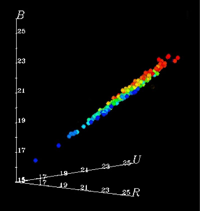Figure 3. Three broadband colours as a function of red-shift, Connolly et al. (1995). [ JPEG | TIFF ]

Before we continue to use photometric red-shift methods for further investigations we will compare the two techniques. In order to do this we have selected a 9 deg² area in the Elais N1 region. The data has been collected as part of the ING's Wide Field Survey (WFS) campaign in the Ug'r'i'z band-passes and reduced via the ING/CASU WFS pipelines (see http://www.ast.cam.ac.uk/~wfcsur/pipeline.html). Object catalogs have been produced and formatted for use with the two methods. The method of Connolly et al. (1995) requires the use of UBRI magnitudes to which the Ug'r'i' were corrected using Fukugita et al. (1996). Magnitudes were also corrected for the effects of atmospheric extinction at the La Palma site (King, 1985). An estimation of reddening was made using Schlegel et al. (1998). The 4096×4096 pixel Lambert projection of dust in the North Galactic Pole was obtained via ftp to Berkeley (ftp deep.berkeley.edu). Using the available IDL interface, an estimation was made and averaged over the Elais region centred at RA 16 10 00 DEC +54 30 00 (J2000). E(B–V) was then converted to the required band-passes.
This same method of magnitude correction was also used for the hyperz code. However, a colour correction was not needed as the code allows you to map in the response of the filters used. Hyperz also accommodates the use of all the Ug'r'i'z wave-bands.
A simple way of testing the methods described is to compare the photometrically determined redshifts with those from direct spectroscopic measurements. Extensive searches of NED and LEDA found fifteen galaxies in the sampled Elais area with predetermined red-shifts. Once these red-shifts have been determined plots of z_spec against z_phot can be made and compared.
Galaxies exhibit a wide variety of morphological types, it's not certain that we can see all of them across the colour ranges, especially faint dwarf galaxies. Looking through the catalogs showed that more sources were present in the g' and r' bands than the U due largely to the poorer limiting magnitude reached in U. These extra sources could not be used with the Connolly method as it does not accommodate null detections. The result is a lower galaxy count (more so at the higher red-shifts). The hyperz method facilitates for effects such as age-metallicity links, the reddening law, flux decrements in the Lyman forest and the cosmological parameters H₀, ₀, when building the synthetic spectra, these null detections are therefore accounted for here.
The mosaic nature of the WFC creates gaps between each chip in the array. Dithering the images or rotating the array on the sky are methods which can be used in order to remove these gaps, but these were not used for the Elais region. Our sample area includes many of these gaps which run all over the region. If it is assumed that the distribution of galaxies within these regions follow that of the hole sample then an estimation of the missing galaxies can be made.
At present we have surveyed the 9 deg²area using the training set method of Connolly (1995). Figure 4 shows the distribution of the galaxy
red-shifts and reflects the increase of galaxies with volume and the sensitivity limit of the survey. Comparison of predetermined galaxy red-shifts with these photometric red-shifts (see Figure 5) suggest that the Connolly relation may need to be trained further to accommodate the different colours used. The dispersion in the fit is z=0.086 compared to a z=0.057 noted by Connolly et al. (1995).

Figure 4. Distribution of galaxy red-shifts within the 9 deg² sampled area. [ GIF | TIFF ] Figure 5. Plot of linear red-shifts against spectroscopic redshifts for objects in the Elais N1 region. [ GIF | TIFF ]

In the near future we will have surveyed the entire 9 deg² area using both methods. Further plots of z_spec versus z_phot will show which method produces more accurate red-shift data, this method then being used to carry out red-shift surveys with INT data and to investigate areas such as the large scale structure more readily.
References:

Astronomical Society of the Pacific Conference Series, 1999, "Photometric Redshifts and High Redshift Galaxies", Volume 191.

Baum, W. A., "Problems of Extra-Galactic Research", IAU Symposium, 15, 390.

Bolzonella, M. et al., "Photometric Redshifts based on standard SED fitting procedures", to appear in A&A, astro-ph/0003380.

Brunner, R. J. et al., 1997, "Towards More Precise Photometric Redshifts: Calibration Via CCD Photometry", ApJ, 482, L21.

Carroll, B. W., Ostlie, D. A., 1996, "An Introduction to Modern Astrophysics", Addison Wesley.

Connolly, A. J. et al., 1995, "Slicing Through Multicolor Space: Galaxy Redshifts From Broadband Photometry", AJ, 110, 2655.

Connolly, A. J. et al., 1995, "Spectral Classification of Galaxies: An Orthogonal Approach", AJ, 110, 1071.

Csabai, I., Connolly, A. J., Szalay, A. S., "Reconstructing Galaxy Spectral Energy Distributions from Broadband Photometry", astro-ph/9910389.

Fukugita, M. et al., 1996, "The Sloan Digital Sky Survey Photometric System", AJ, 111, 1748.

Geller, M. J., and Huchra, J. P., 1989, "Mapping the Universe", Science, 246, 897.

Hogg, D. W. et al., 1998, "A Blind Test of Photometric Redshift Prediction", AJ, 115, 1418.

King, D. L., 1985, "Atmospheric Extinction at the Roque de Los Muchachos Observatory, La Palma", RGO/La Palma Technical Note No. 31.

Koo, D. D., 1985, "Optical Multicolors – A Poor Person's Z Machine for Galaxies", AJ, 90, 418.

Landolt, U., 1992, "UBVRI Photometric Standard Stars in the Magnitude Range 11.5<V<16.0 Around the Celestial Equator", AJ, 104, 1.

Loh, E. D., Spillar, E. J., 1986, "Photometric Reshifts of Galaxies", ApJ, 303, L154.

McMahon, R. G. et al., 1999, "The INT Wide Field Imaging Survey (WFS)", Preprint submitted to Elsevier Preprint.

Moore, B. et al., 1992, "The Topology of the QDOT IRAS Redshift Survey", MNRAS, 256, 477.

Schlegel, D. J. et al., 1998, "Maps of Dust Infrared Emission for Use in Estimation of Reddening and Cosmic Microwave Background Radiation Foregrounds", ApJ, 500, 525.

Slinglend, K. et al., 1998, "The MX Northern Abell Cluster Redshift Survey", APJS, 115, 1.

Wang, Y., Bahcall, N., Turner, E. L., 1998, "A Catalog of Color-Based Redshifts Estimators for z<4 Galaxies in the Hubble Deep Field", AJ, 116, 2081.

Email contact: Dan Batcheldor (dpb@ing.iac.es)

Previous: Lithium Trail Leads Back to the Big Bang Up: Table of Contents Next: First Light of INGRID on the WHT !

GENERAL SCIENCE TELESCOPES AND INSTRUMENTATION OTHER NEWS FROM ING TELESCOPE TIME

© Isaac Newton Group of Telescopes


Figure 1. Distribution of ~4000 galaxies in red-shift space, Geller and Huchra (1989). [ JPEG \| TIFF ]	Figure 2. Distribution of galaxies within 100Mpc of the Milky Way, Moore et al. (1992). [ JPEG \| TIFF ]


Figure 4. Distribution of galaxy red-shifts within the 9 deg² sampled area. [ GIF \| TIFF ]	Figure 5. Plot of linear red-shifts against spectroscopic redshifts for objects in the Elais N1 region. [ GIF \| TIFF ]