INTEGRAL/WYFFOS

• Documentation
• Basic Information
• Spectral Resolutions
• Calibration Information
• Quick Look/Data Reductions

The INTEGRAL manual is still under construction. Here you can find the manual original version.

Click here for the most recent version of the on-line SETUP and Observing Procedures.
 
 

Basic Information

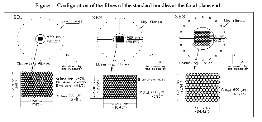
Up to six scientific bundles can be simultaneously mounted in the Swing Plate (SP) ,located in the telescope focal plane area, although in the standard configuration only three are used (called sb1, sb2,and sb3). These bundles are 5.5 m long, while their fibre core diameter (in sky units) is: 0.45 (sb1), 0.9 (sb2), and 2.7 (sb3) arcsec respectively. The bundles are simultaneously connected at the entrance pseudo-slit of the wyffos spectrograph. They can be interchanged very easily, with an overhead of a few seconds.  Hence, depending on the prevailing seeing conditions the instrument can be easily optimized for the scientific program.

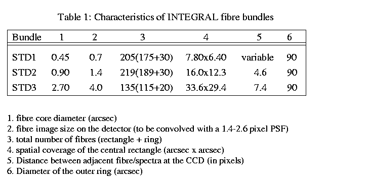
At the focal plane the fibres are arranged in two groups, one forming a rectangle, and the other a ring which is intended for collecting background light (for small-sized objects). Table 1 and Figure 1 show the main characteristics of each bundle.
 
 

Spectral Resolutions

For any particular grating the spectral resolution depends on the fibre bundle as a consequence of the different fibre sizes. Table 2 lists the mean spectral resolution and linear dispersions for different gratings and bundle (reflexion mode). Note that due to the variation of the Wyffos focus over the CCD (which affects the FWHM) the spectral resolution also changes over the CCD.
 
 

Table 2: Spectral Characteristics

	1200 g/mm	600 g/mm	316 g/mm	300 g/mm	ech. Order 7	ech. Order 6	ech. Order 5	ech. Order 4	ech. Order 3
Resolution (STD1) (A)	2.8	6.0	11.8	11
Resolution (STD2) (A)	2.8	6.0	11.8	12.0
Resolution (STD3) (A)	4.8	9.8	19.4	19.6			1.22
Linear Dispersion (A/pix)	1.4	3.07	5.9	6.2			0.35
Spectra Coverage (A)	1445	3140	5837	6144			358

 
 
 

Calibration Information

Arc maps from INTEGRAL on the WHT.
 

Arcs with other bundles and same grating look like close similar. As example: STD2, STD3
 
 

Quick Look/Data Reductions
 

For a quick look of data during your run you can follow the next steps:

1. Turn on the white lamp and take a flat exposure:

                  ICL> ila W in
                  ICL> run integral 2 "flat STD"  -> flat_STD?.imh
    This flat can be use as a reference flat for the observing night. Then, we suggest  rename it to an easy name (e.g. flat_STD?.imh)

2. Type integral in the IRAF environtment to load the INTEGRAL package

3. Use int_apall task to define and extract aperture from the taken flat (flat_STD?.imh) without any reference flat.

4. Take an exposure of your object
                     ICL> run integral 1800 "NGC1068 STD2 5000A"

5. Use int_apall task to extract apertures from your object frame. Put as reference flat your flat_STD?.imh and answer NO when task ask for tracing fibers. The result of this tak should be a file called as your object frame  but with .ms at the end (e.g. r294021.imh -> r294021.ms.imh). This file is a 1124xN pixels image, where N is the number of fibers of the bundle used.

6. Use imarec task to recover your observed object. This task allows to performe a map of an object between two pixels along the dispersion axis. The output of this task is an image that you can display as a common frame (e.g. display image_reconstruction).
 

Information on how to reduce your INTEGRAL data can be found here.
 

Last updated March 2000
Begoña García-Lorenzo (Instrument specialist)
bgarcia@ing.iac.es

Ana M. Pérez-García (Deputy)
aperez@ing.iac.es