Ask the optical engineer to change LIRIS halfwave plates for ISIS
polarizers MF-POL-PAR and MF-POL-PER, if before the run they are not mounted
in the main colour-filter slide in the WHT A&G box.
The ISIS and LIRIS filters are now permanently mounted simultaneously in the A&G box slides. The ISIS MF-POL-PAR and MF-POL-PER polarisers are mounted in the mainfiltnd slide in position 2 (MF-POL-PAR) and position 3 (MF-POL-PER). The LIRIS halfwave plates are mounted in the mainfiltc slide.
A standard configuration is to have the halfwave plate mounted on top of the quarterwave plate,
so that the quarterwave plate is closer to the slit. The quarterwave and halfwave plates
can be interchanged, to optimize a particular application. This has to be done when ISIS is
off the telescope, hence you should find out whether your observer plans to
use such a non-standard configuration and communicate this change to the
optical engineers well in advance.
Setting up the spectrograph for spectropolarimetry
If the two ISIS arms are going to be used for observing, complete the spectropolarimetry
setup for one arm and then proceed in the same way for the other
arm.
Set up ISIS as usual
Follow the
standard procedure to set up ISIS (rotation, tip-tilt, and CCD focus)
with the grating and central wavelength as requested by the PI.
IMPORTANT! Remember that it is NOT recommended to use a dichroic,
therefore do the ISIS set up without the dichroic:
SYS@taurus>bfold 0, to observe in the red arm only
SYS@taurus>bfold 1, to observe in the blue arm only
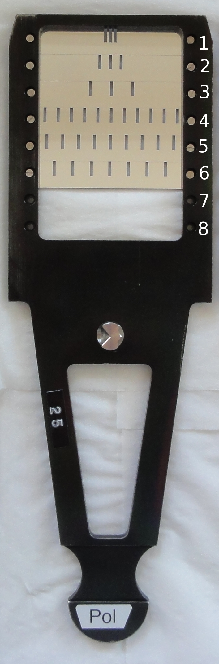
Insert the polarization dekker
After finishing the usual setup, you have to physically insert the
polarization dekker in the dekker slide:
SYS@taurus> dekker 1
SYS@taurus> slit_door open
Go to the WHT dome, open the slit door, pull out the 'Observing' dekker
slide (labeled 'Obs') to take it out and put it back in its box.
Take the 'Polarization' dekker
slide (labelled 'Pol') and introduce it in the dekker unit.
Be careful to arrive to the end of the rail where it should click into place.
Close the slit door securely by snapping softly the locks. Finally, lock the slit door from the ICS:
SYS@taurus> slit_door close
Set the dekker name:
SYS@taurus> setdekkerset polarisation
Put the dekker in correct position (the default option is dekker in position 2):
SYS@taurus> dekker 3
Note that the dekker in 'position 2' is reached by the ICS command 'dekker 3'.
Now click on the 'Update Filters' button in both the 'ISIS Observer' and
'ISIS Eng.' tabs of the Instrument Control Console so that the dekker mask
drop-down menus are updated.
Define the appropriate CCD window
Move the Savart plate into beam:
SYS@taurus> fcp calcite
Move halfwave or quarterwave plate in:
SYS@taurus> hwin, for linear polarimetry
or SYS@taurus> qwin, for circular polarimetry
SYS@taurus> agcomp
SYS@taurus> complamps w
SYS@taurus> flat red 0.5 "window" (adjust exposure time according to ISIS setup)
Display the image in DS9 and define the appropriate window.
In the case of the example here, dekker in position 2, you should see six
stripes of light, the 'ordinary' and 'extraordinary' beams for each of the
three dekker-mask apertures. Ideally, the window should cover the six stripes
of light, and have a margin of about 50 pixels on either side
of the most external stripes. See Fig. 1 as an example.
Once you have defined the window set it as usual, for example:
SYS@taurus> window red 1 "[890:1240,1:4200]"
Fig. 1 - An example of image with a window including a margin of about
50 pixels on either side of the most external stripes.
Check the spectrograph focus
Keep record of the initial ISIS collimator values (from step 2) and give them to
observers. They will need this information in case they are planning
to switch to normal ISIS observations during the run.
With the calcite in the light beam, the spectrograph focus should be about 9200 microns
higher than the one obtained in the standard ISIS set up (step 2). The
reason is that there is now an extra optical element (calcite plate) between
the slit and the collimator, and the spectrograph focal length will change.
In order to stay in anastigmatic region of the spectrograph, we will need to
add about 9200 microns to the previously determined best spectrograph focus.
So, for example, optimal collimator value for the red arm with GG495 and no dichroic should
be rcoll = 10100 + 9200:
SYS@taurus> rcoll 19300
Similarly, optimal collimator value for the red arm without GG495 and no dichroic should
be rcoll = 9300 + 9200 = 18500, and optimal collimator value for the blue
arm should be bcoll = 5100 + 9200 = 14300.
SYS@taurus> slitarc 0.7 (use a fairly small slit width)
SYS@taurus> complamps cune+cuar (check that no ND filter is
deployed in the calibration-lamps unit)
SYS@taurus> arc red 2 "focus"
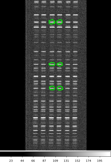
Note that longer exposure times should now be used due to the presence of
the wave plate and the calcite slab. Display the arc image in DS9 and check the
FWHM of several isolated arc lines close to the centre of the
detector for the central ordinary (o) and extraordinary (e) beams (for example, arc lines
marked in green on Fig. 2).
Then move the collimator value in steps of about 500 microns
in both directions, take an arc in each step and measure FWHM of the same
isolated arc lines as before. Repeat until the minimum FWHM in both rays is obtained,
where also a difference of FWHM between o and e rays
should be minimal. This is the final collimator value which should be
used for observations.
Fig. 2 - Arc image where green labels mark example arc lines to
measure the best spectrograph focus.
Find the zero angle of the setup for the required retarder plate
Zero angle is the angle of the retarder plate for which the contrast between the
ordinary (o) and extraordinary (e) beams is maximized. Feed the spectrograph
with linearly polarized light by inserting the MF-POL-PAR polarizer in the
beam:
SYS@taurus> mainfiltnd MF-POL-PAR
Because we are feeding the spectrograph with linearly polarized light, the
theoretical zero angles should be around 45 deg for circular polarimetry and
0 deg for linear polarimetry. However, the respective zero angles in ISIS
are around 50 deg and 8 deg instead.
Besides, these values can vary by up to 4 deg depending
on the grating and central wavelength in use. Table 1 in the section
Useful information lists some zero
angles determined for different set-ups (note that +45 deg is added to the
measured zero angle for circular polarimetry - see the following text about
circular polarization).
Now you should take W-flats around the expected zero angle:
SYS@taurus> complamps w
SYS@taurus> hwp <angle> or qwp <angle>,
to move the required plate to a requested angle between 0-360 deg
SYS@taurus> flat red 2 "angle"
To measure the average brightness use the central o and e rays. You
can use the iraf imstat command on two rectangular regions,
which must have the same size (see Fig. 3). For example:
cl> imstat r123456.fit[1][200:210,1800:2500] for the o ray
cl> imstat r123456.fit[1][240:250,1800:2500] for the e ray
Always use a fairly long region for good statistics on both rays.
Take a note of the average count values and compute the difference. Do the
same at remaining angles and record the angle of the maximum difference
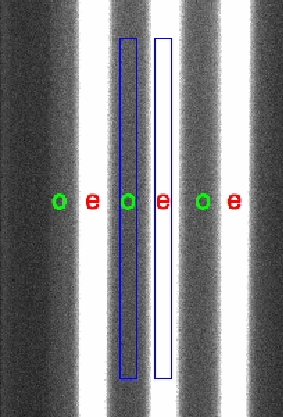
between both rays which will be the zero angle. Fig. 3 - A zoomed region of a flat field taken with the
quarterwave plate at 39 deg. The ordinary (o) and extraordinary (e) rays
are labeled. The blue rectangular regions are used to compute average
brightness values.Linear polarization (using the hwp plate)
Theoretically, for linear-polarization observations, the target should be observed at
the halfwave-plate angles 0, 45, 22.5, and 67.5 degrees.
Hence, you should add +0, +45, +22.5, and +67.5 degrees to the zero angle you have found
and use these angles for science observations by introducing them in
the linear-polarimetry
script at /home/whtobs/isis_scripts/linpolscript.
It is a good practice to check that other plate angles (+22.5, +45, and +67.5) make sense.
With the half-wave plate at 22.5 and 67.5 deg away from the zero angle the difference
in the intensity between the ordinary and extraordinary beams should be
minimal, at 45 deg maximal (see Fig. 4).
Circular polarization (using the qwp plate)
We were feeding the spectrograph with linearly polarized
light when we measured a zero angle (we used the MF-POL-PAR), and therefore
a final zero angle is obtained by adding 45 degrees to the measured angle.
That is, if 50 degrees was the zero angle
with the MF-POL-PAR, then the angle in the script for circular polarimetry should be
50+45=95 degrees.
We will use this angle and +90 degrees in the
circular-polarimetry
script at /home/whtobs/isis_scripts/cirpolscript. Note that instead of
95 and 185 degrees one can use also 5 and 95 degrees for the observations.
When you are finished, remember to remove the MF-POL-PAR filter out of the beam:
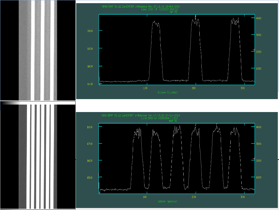
SYS@taurus> mainfiltnd out Fig. 4 - Image taken using the halfwave plate, showing the expected difference between
the zero angle (top) and the zero angle + 22.5 degrees (bottom).
The table below summarizes the expected ISIS wave plate angles when doing linear
and circular spectropolarimetry observations.
The insertion of the halfwave plate after the acquisition (without the
halfwave plate) does not move the star image relative to the slit, within
the accuracy of acquisition of ~ 0.1 arcsec.
After a spectropolarimetry run
If you want to configure ISIS from a spectropolarimetry into a longslit mode,
proceed as following:
Physically change dekkers: take the polarization dekker out and insert
the observing dekker. Then change the dekker name:
SYS@taurus> setdekkerset observing
Remove polarization optics from a light path:
SYS@taurus> hwout (qwout), moves halfwave (quarterwave) plate out
SYS@taurus> fcp_out, moves the Savart plate out of beam
SYS@taurus> mainfiltnd 1, removes polarizer in the main colour-filter
unit
Set usual collimator values:
SYS@taurus> rcoll 10960 for observations in the red arm with a
dichroic and GG495
SYS@taurus> bcoll 5100 for observations in the blue arm.
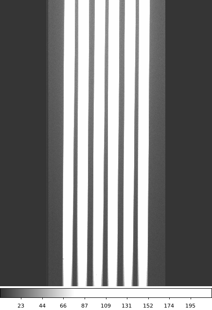
Each bit of dust on the calcite block generates two dark streaks on the image,
in the ordinary and extraordinary ray, which at first look like remanence after
a dekker exposure. An example of the dust on the calcite block can be seen
in the image below.
If you encounter dust on the calcite block, please let the IS and the
optical engineer know. Otherwise, the calcite block should be serviced at
regular intervals, every 2 to 3 years, due to the optical gel drying
out. Fig. 5 - Tungsten-lamp flat taken with a calcite block and without a
dekker in the beam. There is a light loss of 10 % in the left-hand dip,
and few % in the right-hand dip, due to the dust on the calcite block.
Zero angles measured for different set-ups
Zero angles determined for different set-ups are listed in the table
below.


